The Free Lunch Effect: The Value of Decoupling Diversification and Risk - August 2014
Salient Partners


Description
The Free Lunch Effect:
The Value of Decoupling Diversification and Risk
August 2014
Roberto Croce, Ph.D.
Rusty Guinn
Travis Robinson
. Salient Whitepaper #2014-01
This information is being provided to you by Salient Capital Advisors, LLC, and is intended solely for educational purposes. This is neither an offer to sell
nor a solicitation of an offer to buy any securities. No other distribution or use of these materials has been authorized. The opinions expressed in these
materials represent the personal views of the investment professionals of Salient Capital Advisors, LLC and is based on their broad based investment
knowledge, experience, research and analysis.
It must be noted, however, that no one can accurately predict the future of the market with certainty or guarantee future investment performance. Past performance is not a guarantee of future results. Information is for U.S.
residents only. Certain statements in this communication are forward-looking statements of Salient Capital Advisors, LLC. The forward-looking statements and other views expressed herein are as of the date of this letter. Actual future results or occurrences may differ significantly from those anticipated in any forward-looking statements, and there is no guarantee that any predictions will come to pass. The views expressed herein are subject to change at any time, due to numerous market and other factors.
The Advisor disclaims any obligation to update publicly or revise any forward-looking statements or views expressed herein. There can be no assurance that the Strategy will achieve its investment objectives. The value of any strategy will fluctuate with the value of the underlying securities. Please note that the returns presented in this paper are the result of a hypothetical investment framework.
Backtested performance is NOT an indicator of future actual results and do the results above do NOT represent returns that any investor actually attained. Backtested results are calculated by the retroactive application of a model constructed on the basis of historical data and based on assumptions integral to the model which may or may not be testable and are subject to losses. Certain assumptions have been made for modeling purposes and are unlikely to be realized.
No representations and warranties are made as to the reasonableness of the assumptions. Changes in these assumptions may have a material impact on the backtested returns presented. This information is provided for illustrative purposes only.
Backtested performance is developed with the benefit of hindsight and has inherent limitations. Specifically, backtested results do not reflect actual trading or the effect of material economic and market factors on the decisionmaking process. Since trades have not actually been executed, results may have under- or over-compensated for the impact, if any, of certain market factors, such as lack of liquidity, and may not reflect the impact that certain economic or market factors may have had on the decision-making process. Further, backtesting allows the security selection methodology to be adjusted until past returns are maximized.
Actual performance may differ significantly from backtested performance. Backtested results are adjusted to reflect the reinvestment of dividends and other income. The backtested results do not include the effect of backtested transaction costs, management fees, performance fees or expenses, if applicable.
No cash balance or cash flow is included in the calculation. There are special risks associated with an investment in commodities and futures, including market price fluctuations, regulatory changes, interest rate changes, credit risk, economic changes and the impact of adverse political or financial factors. Transactions in futures are speculative and carry a high degree of risk. Research and advisory services are provided by Salient Capital Advisors, LLC, a wholly owned subsidiary of Salient Partners, L.P. and a U.S.
Securities and Exchange Commission Registered Investment Adviser. Registration as an Investment Adviser does not imply any level of skill or training. Salient research has been prepared without regard to the individual financial circumstances and objectives of persons who receive it.
Salient recommends that investors independently evaluate particular investments and strategies, and encourage investors to seek the advice of a financial advisor. The appropriateness of a particular investment or strategy will depend on an investor’s individual circumstances and objectives. No investment strategy can guarantee performance results. All references to historic returns are based on the hypothetical performance of the strategy as backtested for research purposes.
“Expected returns” refer to the general expectations of risk premia arising from various asset classes in the context if a risk-return relationship and are in no way intended to be forward looking projections. Diversification does not ensure a profit or guarantee against loss. Salient is the trade name for Salient Partners, L.P., which together with its subsidiaries provides asset management and advisory services. Insurance products offered through Salient Insurance Agency, LLC (Texas license #1736192). Trust services provided by Salient Trust Co., LTA.
Securities offered through Salient Capital, L.P., a registered broker-dealer and Member FINRA, SIPC. Each of Salient Insurance Agency, LLC, Salient Trust Co., LTA, and Salient Capital, L.P., is a subsidiary of Salient Partners, L.P. © Salient Capital Advisors, LLC, 2014. Authors: Roberto Croce, Ph.D.; Rusty Guinn; Travis Robinson 2 . Salient Whitepaper #2014-01 Summary Whether professional or not, many investors are familiar with the most well-advertised feature of diversification, namely that it may reduce the risk of a portfolio while maintaining the same level of expected return. This concept is so attractive and so intuitive that it is easy to see diversification and the reduction of risk as the same thing. They are not. In this piece, we will discuss why thinking about diversification and risk independently may help investors to build more efficient portfolios. In particular, we introduce a way to think about the diversification potential of portfolios, or the Free Lunch Effect.
1 We will also explore certain common allocation methods, including traditional “balanced” portfolios, and the assumptions for the returns of different markets that are embedded within them. We highlight several key lessons and observations from this exercise:  Adding assets that reduce risk does not mean an investor is diversifying  While they may be a comfortable fallback, traditional balanced portfolios often force investors into unintended bets  Higher volatility diversifiers may be among the most powerful tools an investor has Risk and Diversification Let us start by considering a sample stock portfolio, in which an investor buys the S&P 500 Index, perhaps through an exchange-traded fund (ETF) or mutual fund. Using data from July 1984 to June 2014, we observe that this investment would have had a volatility of 15.3%. There are many ways to look at risk – some good, some bad, and none perfect.
We think that volatility does a good job of contributing to an investor’s perspective of the potential for loss or gain - the uncertainty of value and will use it throughout this piece. One of the first actions many investors often take to diversify and/or reduce the risk of such a portfolio is to invest a portion of this stock portfolio in bonds. A traditional “balanced” approach is to invest 40% in bonds and 60% in stocks. For the purposes of this analysis, stocks will be represented by the S&P 500 and bonds will be represented by the commonly used Barclays Aggregate Bond Index.
Over the last 30 years this portfolio would have had a volatility of 9.5%, significantly less risk than that of a portfolio that held only stocks – 5.7% less, to be specific. It is tempting (and popular) to think of this reduction in risk as the benefit of diversification. It is also misleading. To understand why, we have to understand the reason volatility – our measure of risk – declined when we added bonds.
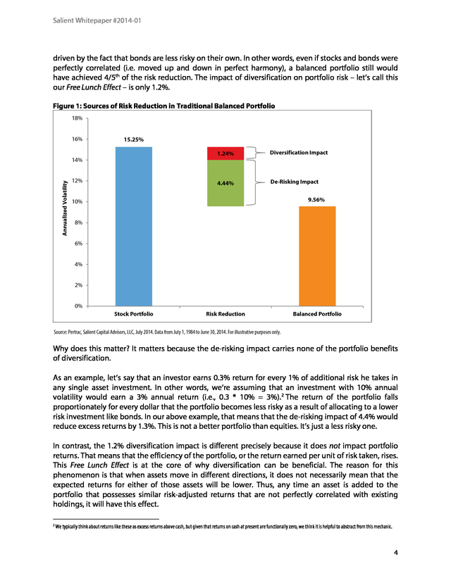
There are two reasons why blending stocks and bonds, or any other pair of assets or portfolios, may result in reduced risk. One of those is indeed the benefit of diversification, the impact that portfolios receive from incorporating investments that do not always move together. The second, and in this case more important, reason why a balanced portfolio is often less risky than a stock only portfolio is that bonds themselves are less risky than stocks. In Figure 1 on the following page we show how much each of these two effects drove the reduction in risk of a balanced portfolio.
In practice, approximately 1/5th of the reduction in volatility from a 100% stock portfolio to a balanced portfolio actually came from diversification. The remaining 4/5th was 1 The Free Lunch Effect is a term coined by the authors to describe the reduction in portfolio risk that accrues to portfolios because asset correlations are less than one. One of the purposes of this paper is to make plain the distinction between risk reduction occurring due to imperfect correlation versus the reduction due to allocating to assets with lower risk.
We call this decomposition of changes in risk into the Cash Effect and the Free Lunch Effect. 3 . Salient Whitepaper #2014-01 driven by the fact that bonds are less risky on their own. In other words, even if stocks and bonds were perfectly correlated (i.e. moved up and down in perfect harmony), a balanced portfolio still would have achieved 4/5th of the risk reduction. The impact of diversification on portfolio risk – let’s call this our Free Lunch Effect – is only 1.2%. Figure 1: Sources of Risk Reduction in Traditional Balanced Portfolio 18% 16% 15.25% 1.24% Annualized Volatility 12% Diversification Impact 4.44% 14% De-Risking Impact 9.56% 10% 8% 6% 4% 2% 0% Stock Portfolio Risk Reduction Balanced Portfolio Source: Pertrac, Salient Capital Advisors, LLC, July 2014.
Data from July 1, 1984 to June 30, 2014. For illustrative purposes only. Why does this matter? It matters because the de-risking impact carries none of the portfolio benefits of diversification. As an example, let’s say that an investor earns 0.3% return for every 1% of additional risk he takes in any single asset investment. In other words, we’re assuming that an investment with 10% annual volatility would earn a 3% annual return (i.e., 0.3 * 10% = 3%).
2 The return of the portfolio falls proportionately for every dollar that the portfolio becomes less risky as a result of allocating to a lower risk investment like bonds. In our above example, that means that the de-risking impact of 4.4% would reduce excess returns by 1.3%. This is not a better portfolio than equities.
It’s just a less risky one. In contrast, the 1.2% diversification impact is different precisely because it does not impact portfolio returns. That means that the efficiency of the portfolio, or the return earned per unit of risk taken, rises. This Free Lunch Effect is at the core of why diversification can be beneficial. The reason for this phenomenon is that when assets move in different directions, it does not necessarily mean that the expected returns for either of those assets will be lower.
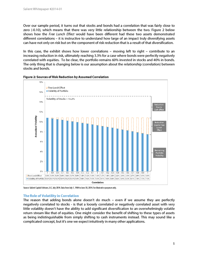
Thus, any time an asset is added to the portfolio that possesses similar risk-adjusted returns that are not perfectly correlated with existing holdings, it will have this effect. 2 We typically think about returns like these as excess returns above cash, but given that returns on cash at present are functionally zero, we think it is helpful to abstract from this mechanic. 4 . Salient Whitepaper #2014-01 Over our sample period, it turns out that stocks and bonds had a correlation that was fairly close to zero (-0.10), which means that there was very little relationship between the two. Figure 2 below shows how the Free Lunch Effect would have been different had these two assets demonstrated different correlations – it is instructive to understand how large of an impact truly diversifying assets can have not only on risk but on the component of risk reduction that is a result of that diversification. In this case, the exhibit shows how lower correlations – moving left to right – contribute to an increasing reduction in risk, ultimately reaching 3.3% for a case where bonds were perfectly negatively correlated with equities. To be clear, the portfolio remains 60% invested in stocks and 40% in bonds. The only thing that is changing below is our assumption about the relationship (correlation) between stocks and bonds. Figure 2: Sources of Risk Reduction by Assumed Correlation Source: Salient Capital Advisors, LLC, July 2014. Data from July 1, 1984 to June 30, 2014.
For illustrative purposes only. The Role of Volatility in Correlation The reason that adding bonds alone doesn’t do much – even if we assume they are perfectly negatively correlated to stocks - is that a loosely correlated or negatively correlated asset with very little volatility doesn’t have the ability to add significant diversification to an overwhelmingly volatile return stream like that of equities. One might consider the benefit of shifting to these types of assets as being indistinguishable from simply shifting to cash instruments instead. This may sound like a complicated concept, but it’s one we expect intuitively in many other applications. 5 .
Salient Whitepaper #2014-01 Consider, for example, a small ensemble of three musicians. You are tasked with directing your little group to play a beautiful chord of three notes, beginning with our trumpet player, who blares out an offensively loud high C. You now have a choice of how to build the chord. You could certainly have your second and third players pick up a clarinet or violin, but even the non-musical among us can see the issue here.
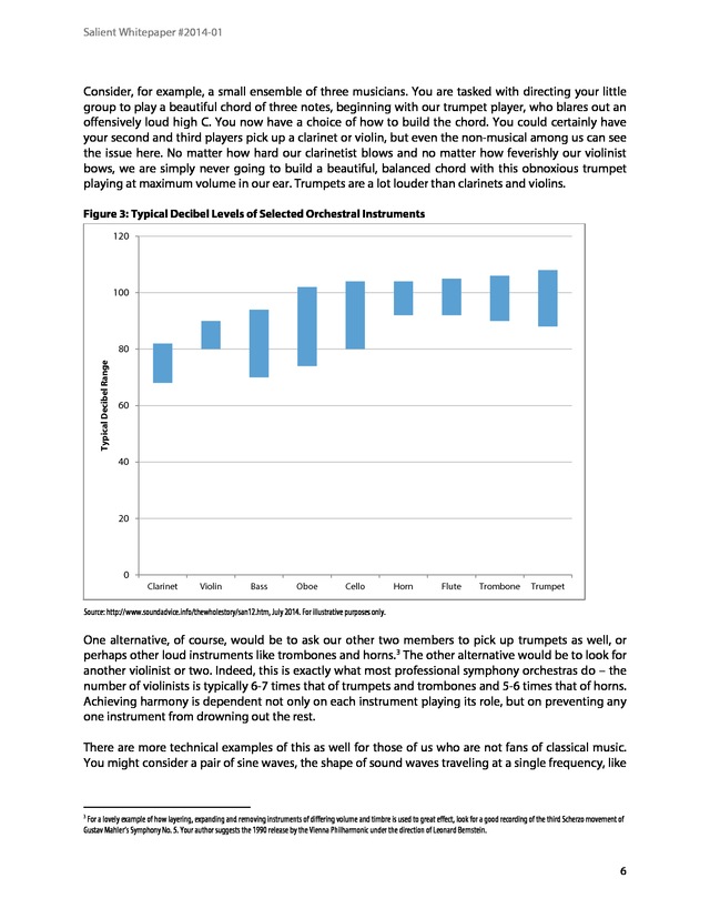
No matter how hard our clarinetist blows and no matter how feverishly our violinist bows, we are simply never going to build a beautiful, balanced chord with this obnoxious trumpet playing at maximum volume in our ear. Trumpets are a lot louder than clarinets and violins. Figure 3: Typical Decibel Levels of Selected Orchestral Instruments 120 100 Typical Decibel Range 80 60 40 20 0 Clarinet Violin Bass Oboe Cello Horn Flute Trombone Trumpet Source: http://www.soundadvice.info/thewholestory/san12.htm, July 2014. For illustrative purposes only. One alternative, of course, would be to ask our other two members to pick up trumpets as well, or perhaps other loud instruments like trombones and horns.
3 The other alternative would be to look for another violinist or two. Indeed, this is exactly what most professional symphony orchestras do – the number of violinists is typically 6-7 times that of trumpets and trombones and 5-6 times that of horns. Achieving harmony is dependent not only on each instrument playing its role, but on preventing any one instrument from drowning out the rest. There are more technical examples of this as well for those of us who are not fans of classical music. You might consider a pair of sine waves, the shape of sound waves traveling at a single frequency, like 3 For a lovely example of how layering, expanding and removing instruments of differing volume and timbre is used to great effect, look for a good recording of the third Scherzo movement of Gustav Mahler’s Symphony No. 5.
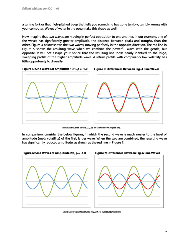
Your author suggests the 1990 release by the Vienna Philharmonic under the direction of Leonard Bernstein. 6 . Salient Whitepaper #2014-01 a tuning fork or that high-pitched beep that tells you something has gone terribly, terribly wrong with your computer. Waves of water in the ocean take this shape as well. Now imagine that two waves are moving in perfect opposition to one another. In our example, one of the waves has significantly greater amplitude, the distance between peaks and troughs, than the other. Figure 4 below shows the two waves, moving perfectly in the opposite direction.
The red line in Figure 5 shows the resulting wave when we combine the powerful wave with the gentle, but opposite. It will not escape your notice that the resulting line looks nearly identical to the large, sweeping profile of the higher amplitude wave. A return profile with comparably low volatility has little opportunity to diversify. Figure 4: Sine Waves of Amplitude 10:1, ρ = -1.0 Figure 5: Differences Between Fig.
4 Sine Waves Source: Salient Capital Advisors, LLC, July 2014. For illustrative purposes only. In comparison, consider the below figures, in which the second wave is much nearer to the level of amplitude (read: volatility) of the first, larger wave. When the two are combined, the resulting wave has significantly reduced amplitude, as shown as the red line in Figure 7. Figure 6: Sine Waves of Amplitude 2:1, ρ = -1.0 Figure 7: Differences Between Fig.
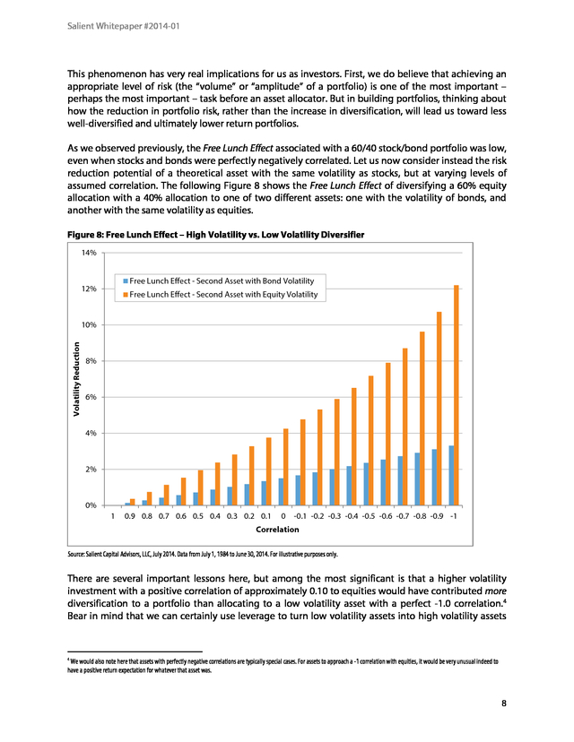
6 Sine Waves Source: Salient Capital Advisors, LLC, July 2014. For illustrative purposes only. 7 . Salient Whitepaper #2014-01 This phenomenon has very real implications for us as investors. First, we do believe that achieving an appropriate level of risk (the “volume” or “amplitude” of a portfolio) is one of the most important – perhaps the most important – task before an asset allocator. But in building portfolios, thinking about how the reduction in portfolio risk, rather than the increase in diversification, will lead us toward less well-diversified and ultimately lower return portfolios. As we observed previously, the Free Lunch Effect associated with a 60/40 stock/bond portfolio was low, even when stocks and bonds were perfectly negatively correlated. Let us now consider instead the risk reduction potential of a theoretical asset with the same volatility as stocks, but at varying levels of assumed correlation.
The following Figure 8 shows the Free Lunch Effect of diversifying a 60% equity allocation with a 40% allocation to one of two different assets: one with the volatility of bonds, and another with the same volatility as equities. Figure 8: Free Lunch Effect – High Volatility vs. Low Volatility Diversifier 14% Free Lunch Effect - Second Asset with Bond Volatility 12% Free Lunch Effect - Second Asset with Equity Volatility Volatility Reduction 10% 8% 6% 4% 2% 0% 1 0.9 0.8 0.7 0.6 0.5 0.4 0.3 0.2 0.1 0 -0.1 -0.2 -0.3 -0.4 -0.5 -0.6 -0.7 -0.8 -0.9 -1 Correlation Source: Salient Capital Advisors, LLC, July 2014. Data from July 1, 1984 to June 30, 2014.
For illustrative purposes only. There are several important lessons here, but among the most significant is that a higher volatility investment with a positive correlation of approximately 0.10 to equities would have contributed more diversification to a portfolio than allocating to a low volatility asset with a perfect -1.0 correlation.4 Bear in mind that we can certainly use leverage to turn low volatility assets into high volatility assets 4 We would also note here that assets with perfectly negative correlations are typically special cases. For assets to approach a -1 correlation with equities, it would be very unusual indeed to have a positive return expectation for whatever that asset was. 8 . Salient Whitepaper #2014-01 (“adding some violins”), but in either case, the point is that adding good diversifiers that match the risk of equities is more powerful than adding diversifiers that cannot. Diversification and Return Efficiency While we have reviewed how investors may maximize the Free Lunch Effect, we have only briefly touched upon why we believe this should be important to investors. As we alluded to before, the Free Lunch Effect is the mechanism through which diversification may increase a portfolio’s reward versus risk. That means it’s time for a refresher on Markowitz and Modern Portfolio Theory (“MPT”) (Markowitz, 1952). Example 1: Perfectly Correlated Assets with Different Volatilities Let us first consider an example in which we are investing in two assets. The first is a high risk asset – let’s call it “Asset A” – with annual volatility of 20% and an expected return of 10%.
The second is a low risk asset – let’s call this one “Asset B” – with annual volatility of 4% and an expected return of 2%. While they have different levels of risk, these two assets are otherwise perfectly correlated. They move consistently up and down together. What happens when we invest in a 50/50 mix of these two portfolios? The answer: the resulting portfolio exhibits a volatility of 12% and an expected return of 6%. Remember that the expected return for a portfolio is always a weighted average of the expected returns of the underlying assets.
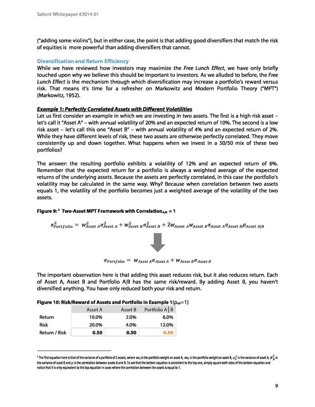
Because the assets are perfectly correlated, in this case the portfolio’s volatility may be calculated in the same way. Why? Because when correlation between two assets equals 1, the volatility of the portfolio becomes just a weighted average of the volatility of the two assets. Figure 9: 5 Two-Asset MPT Framework with CorrelationA|B = 1 2 ðœŽ2 ð‘ƒð‘œð‘Ÿð‘¡ð‘“ð‘œð‘™ð‘–𑜠= 𑤠ð´ð‘ ð‘ ð‘’ð‘¡ ð´ 2 ðœŽ2 ð´ð‘ ð‘ ð‘’ð‘¡ ð´ + 𑤠ð´ð‘ ð‘ ð‘’ð‘¡ ðµ ðœŽ2 ð´ð‘ ð‘ ð‘’ð‘¡ ðµ + 2𑤠ð´ð‘ ð‘ ð‘’ð‘¡ ð´ 𑤠ð´ð‘ ð‘ ð‘’ð‘¡ ðµ 𜎠ð‘ƒð‘œð‘Ÿð‘¡ð‘“ð‘œð‘™ð‘–𑜠= 𑤠ð´ð‘ ð‘ ð‘’ð‘¡ ð´ 𜎠ð´ð‘ ð‘ ð‘’ð‘¡ ð´ + 𑤠ð´ð‘ ð‘ ð‘’ð‘¡ ðµ 𜎠ð´ð‘ ð‘ ð‘’𑡠𜎠ð´ð‘ ð‘ ð‘’ð‘¡ ð´ 𜎠ð´ð‘ ð‘ ð‘’ð‘¡ ðµ 𜌠ð´ð‘ ð‘ ð‘’ð‘¡ ð´|ðµ ðµ The important observation here is that adding this asset reduces risk, but it also reduces return. Each of Asset A, Asset B and Portfolio A|B has the same risk/reward.
By adding Asset B, you haven’t diversified anything. You have only reduced both your risk and return. Figure 10: Risk/Reward of Assets and Portfolio in Example 1(ρab=1) Asset A Asset B Portfolio A│B Return 10.0% 2.0% 6.0% Risk 20.0% 4.0% 12.0% Return / Risk 0.50 0.50 0.50 The first equation here is that of the variance of a portfolio of 2 assets, where wA is the portfolio weight on asset A, wB is the portfolio weight on asset B, 𜎠2 is the variance of asset A, 𜎠ðµ is ð´ the variance of asset B and ρ is the correlation between assets A and B. To see that the bottom equation is consistent to the top one, simply square both sides of the bottom equation and notice that it is only equivalent to the top equation in cases where the correlation between the assets is equal to 1. 5 2 9 .
Salient Whitepaper #2014-01 Example 2: Uncorrelated Assets with Different Volatilities The above is clearly an exaggerated example, but we believe it’s not far from reality for many ways in which many investors attempt to diversify. Certain hedge fund strategies or high yield investment strategies, for example, demonstrate very high correlations with equities but at lower levels of risk. There may be an expectation of a higher return/risk for those investments, of course, an assumption which we will place in context of the Free Lunch Effect later in this paper. More frequently, investors will encounter examples where they attempt to combine two assets which have different volatilities and more moderate correlations. Let us then consider an example in which our assets have volatilities and expected returns identical to what we described in Example 1: Asset A have a volatility of 20% and expected return of 10%, while Asset B have a volatility of 4% and expected return of 2%. Instead of a correlation of 1 between the two assets, however, let’s assume a correlation of zero. As before, the portfolio’s expected returns are 6%, a weighted average of the expected returns of Asset A and Asset B.
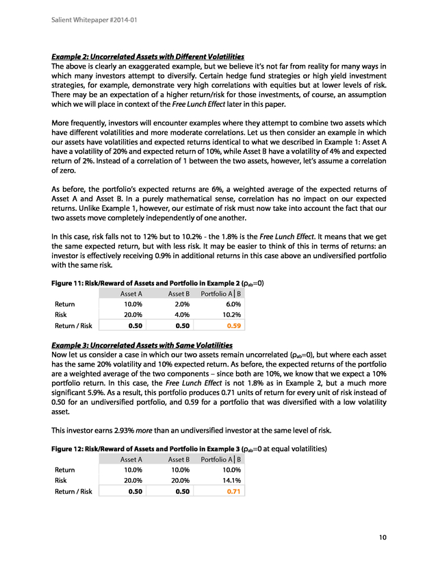
In a purely mathematical sense, correlation has no impact on our expected returns. Unlike Example 1, however, our estimate of risk must now take into account the fact that our two assets move completely independently of one another. In this case, risk falls not to 12% but to 10.2% - the 1.8% is the Free Lunch Effect. It means that we get the same expected return, but with less risk.
It may be easier to think of this in terms of returns: an investor is effectively receiving 0.9% in additional returns in this case above an undiversified portfolio with the same risk. Figure 11: Risk/Reward of Assets and Portfolio in Example 2 (ρab=0) Asset A Asset B Portfolio A│B Return 10.0% 2.0% 6.0% Risk Return / Risk 20.0% 4.0% 10.2% 0.50 0.50 0.59 Example 3: Uncorrelated Assets with Same Volatilities Now let us consider a case in which our two assets remain uncorrelated (ρab=0), but where each asset has the same 20% volatility and 10% expected return. As before, the expected returns of the portfolio are a weighted average of the two components – since both are 10%, we know that we expect a 10% portfolio return. In this case, the Free Lunch Effect is not 1.8% as in Example 2, but a much more significant 5.9%.
As a result, this portfolio produces 0.71 units of return for every unit of risk instead of 0.50 for an undiversified portfolio, and 0.59 for a portfolio that was diversified with a low volatility asset. This investor earns 2.93% more than an undiversified investor at the same level of risk. Figure 12: Risk/Reward of Assets and Portfolio in Example 3 (ρab=0 at equal volatilities) Asset A Asset B Portfolio A│B Return 10.0% 10.0% 10.0% Risk 20.0% 20.0% 14.1% Return / Risk 0.50 0.50 0.71 10 . Salient Whitepaper #2014-01 Implicit Expectations of Non-Diversified Investors In addition to providing a clearer view into a portfolio’s potential return efficiency, the Free Lunch Effect also provides a point of comparison when one begins to consider different views on the risk/reward potential of different asset classes. To this point, we have only considered analysis of risks, or alternatively assumed that each investment had the same Sharpe Ratio. As demonstrated previously, the potential benefit of the Free Lunch Effect is identified by multiplying the effect’s magnitude by the weighted average Sharpe Ratio of the portfolio’s constituents. In other words, by diversifying, you still get the potential “risk/reward” benefit of the units of risk you aren’t taking. If considered in light of the equal Sharpe Ratio assumption, this identity would consistently lead an investor to identify and invest in the most well diversified portfolio possible.
This is the assumption we have made thus far in this piece, and while simplistic, it turns out that the assumption has been approximately true over long historical periods. As pointed out in a prior piece, the longterm Sharpe Ratio of U.S. Treasury Bonds (0.24), Commodities (0.28) and U.S.
Equities (0.28) are very similar (“Risk Parity For the Long Run”, Partridge & Croce, 2012). Especially over shorter periods, this may be an unrealistic assumption, for a couple of reasons. First, it is impossible to know with certainty how much of this diversification benefit an investor may receive in the future. Correlations and volatility can be challenging to forecast.
Second, investors may believe over a particular time horizon that the potential risk/reward payoff will be different among assets in a way that can be predicted. This second belief is very common. It is our contention, however, that many investors are implicitly expressing much more of a view on relative risk/reward efficiency of asset classes than they may believe. For instance, let us consider an example of two assets with the same volatility: the S&P 500 and exposure to the Barclays Aggregate Bond Index that has been levered to get it to the same level of risk (it takes about 5 units of bonds to get to the same level of volatility as stocks). Assuming an equal Sharpe Ratio between these two assets, a 50/50 portfolio is provably optimal in risk-adjusted terms.
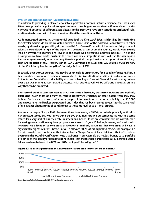
But what if we don’t believe that investors will be compensated with the same return for every unit of risk they take in stocks and bonds? If we are confident we are correct, then increasing one allocation may be appropriate. As shown in Figure 13 below, however, an investor who increases his allocation to one asset or another is implicitly assuming that one asset will have a significantly higher relative Sharpe Ratio. To allocate 100% of his capital to stocks, for example, an investor would need to believe that stocks had a Sharpe Ratio at least 1.4 times that of bonds to overcome the loss of diversification.
Note that bonds in our example are not just bonds, but a portfolio of 5 units of the Barclays Aggregate Bond Index. That means that a traditional 60/40 portfolio would fall somewhere between the 80% and 90% stock portfolio in Figure 13. Figure 13: Implicit Expectations on Relative Risk/Reward Efficiency of Stocks and Bonds 140% 120% 100% 80% 100% 90B/10S 80B/20S 70B/30S 60B/40S 50B/50S 40B/60S 30B/70S 20B/80S 10B/90S 100% Bonds Stocks Implicit Bond Sharpe Premium Implicit Stock Sharpe Premium Source: Bloomberg, Salient Capital Advisors, LLC, July 2014. For illustrative purposes only. 11 .
Salient Whitepaper #2014-01 Said another way, given the historical relationship between stocks and bonds, an investor in a traditional 60/40 portfolio is not expressing a neutral point of view. The investor is implicitly expressing a view that stocks will earn at least 30% more return per unit of risk taken than bonds. We are skeptical that this would be the outcome from a rigorous strategic asset allocation exercise, but we are even more concerned that many investors may not be aware that they are taking this view. Implications for Various Diversification Strategies Since the most traditional approaches to portfolio diversification appear to leave a great deal of diversification potential on the table, we believe it is reasonable to consider the alternatives. As demonstrated in the prior section, leveraging exposure to the most diversifying assets – sovereign bonds, for example - is a straightforward way to achieve better diversification of equity portfolios without scaling down risk in a way that would reduce returns; however, many investors have varying levels of comfort with this concept.
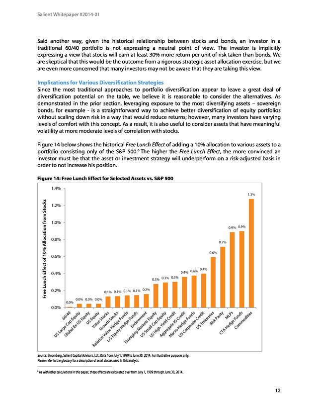
As a result, it is also useful to consider assets that have meaningful volatility at more moderate levels of correlation with stocks. Figure 14 below shows the historical Free Lunch Effect of adding a 10% allocation to various assets to a portfolio consisting only of the S&P 500. 6 The higher the Free Lunch Effect, the more convinced an investor must be that the asset or investment strategy will underperform on a risk-adjusted basis in order to not increase his position. Figure 14: Free Lunch Effect for Selected Assets vs. S&P 500 1.4% Free Lunch Effect of 10% Allocation from Stocks 1.3% 1.2% 1.0% 0.9% 0.9% 0.8% 0.7% 0.6% 0.6% 0.4% 0.4% 0.4% 0.4% 0.3% 0.3% 0.3% 0.2% 0.1% 0.1% 0.1% 0.1% 0.2% 0.0% 0.0% 0.0% 0.0% 0.0% Source: Bloomberg, Salient Capital Advisors, LLC.
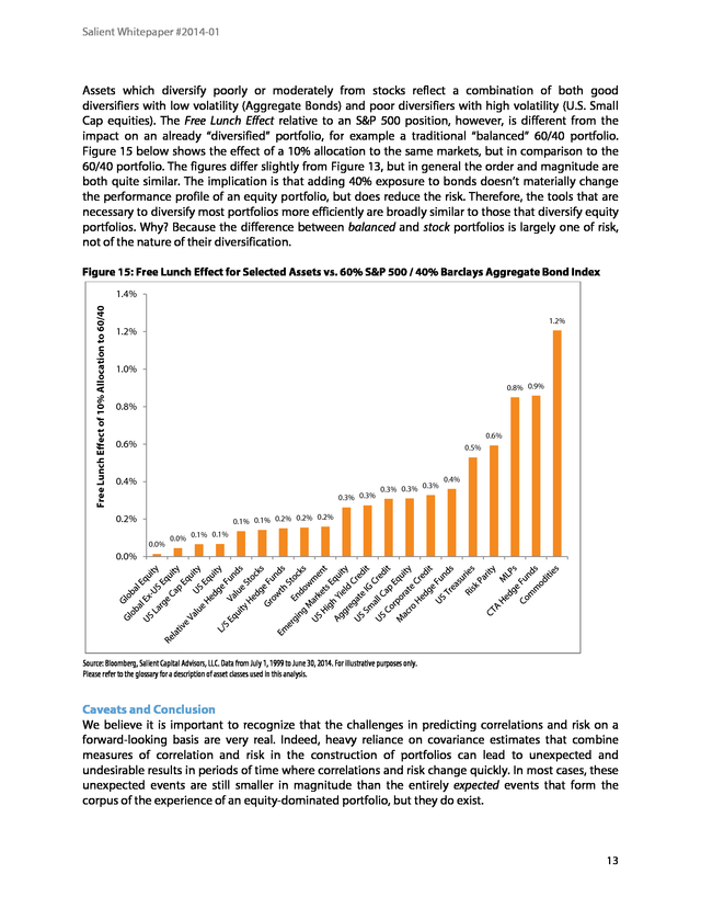
Data from July 1, 1999 to June 30, 2014. For illustrative purposes only. Please refer to the glossary for a description of asset classes used in this analysis. 6 As with other calculations in this paper, these effects are calculated over from July 1, 1999 through June 30, 2014. 12 . Salient Whitepaper #2014-01 Assets which diversify poorly or moderately from stocks reflect a combination of both good diversifiers with low volatility (Aggregate Bonds) and poor diversifiers with high volatility (U.S. Small Cap equities). The Free Lunch Effect relative to an S&P 500 position, however, is different from the impact on an already “diversified” portfolio, for example a traditional “balanced” 60/40 portfolio. Figure 15 below shows the effect of a 10% allocation to the same markets, but in comparison to the 60/40 portfolio. The figures differ slightly from Figure 13, but in general the order and magnitude are both quite similar.
The implication is that adding 40% exposure to bonds doesn’t materially change the performance profile of an equity portfolio, but does reduce the risk. Therefore, the tools that are necessary to diversify most portfolios more efficiently are broadly similar to those that diversify equity portfolios. Why? Because the difference between balanced and stock portfolios is largely one of risk, not of the nature of their diversification. Figure 15: Free Lunch Effect for Selected Assets vs.
60% S&P 500 / 40% Barclays Aggregate Bond Index Free Lunch Effect of 10% Allocation to 60/40 1.4% 1.2% 1.2% 1.0% 0.8% 0.9% 0.8% 0.6% 0.6% 0.5% 0.4% 0.3% 0.3% 0.3% 0.3% 0.3% 0.4% 0.2% 0.1% 0.1% 0.2% 0.2% 0.2% 0.0% 0.1% 0.0% 0.1% 0.0% Source: Bloomberg, Salient Capital Advisors, LLC. Data from July 1, 1999 to June 30, 2014. For illustrative purposes only. Please refer to the glossary for a description of asset classes used in this analysis. Caveats and Conclusion We believe it is important to recognize that the challenges in predicting correlations and risk on a forward-looking basis are very real.
Indeed, heavy reliance on covariance estimates that combine measures of correlation and risk in the construction of portfolios can lead to unexpected and undesirable results in periods of time where correlations and risk change quickly. In most cases, these unexpected events are still smaller in magnitude than the entirely expected events that form the corpus of the experience of an equity-dominated portfolio, but they do exist. 13 . Salient Whitepaper #2014-01 Yet we remain convinced that while predicting risk is difficult, predicting returns, especially over short periods of time, is far more difficult. We believe that shrewd asset allocators should at a minimum ask themselves whether they are sufficiently confident in their preference for one asset over another as to forgo the benefits of the Free Lunch Effect. We believe that allocators would be well-served by challenging the role of low volatility diversifiers in otherwise high volatility portfolios. While low volatility hedge fund strategies and various corporate bond strategies may appear to diversify, we believe that for many portfolios they function primarily as “de-risking” investments, not diversifying investments. Our research shows that higher volatility diversifiers can be powerful – among them, we believe Managed Futures, Commodities, MLPs, Risk Parity strategies and, yes, Treasury Bonds are among the most effective. We continue to believe that many investors may benefit from increasing their allocations to these strategies.
Whether they do so or not, we believe many investors will gain from thinking about diversification as a distinct and desirable portfolio trait, separate from their view on risk. 14 . Salient Whitepaper #2014-01 Appendix: Data and Methodologies “stocks” in this analysis refers to the S&P 500 Total Return Index. “bonds” in this analysis refers to the Barclays Aggregate Bond Index. The risk-free rate refers to the return on 3-month T-bills, as accessed via Bloomberg. All data accumulated as of June 30, 2014. Bibliography Markowitz, H. (1952). Portfolio Selection. Journal of Finance, 77-91. Partridge, L., & Croce, R.
(2012). Risk Parity for the Long Run. Houston: Salient Partners, L.P. Glossary Stocks: S&P 500 Total Return Index - An unmanaged, capitalization-weighted index comprising publicly traded common stocks issued by companies in various industries.
The S&P 500 Index is widely recognized as the leading broad-based measurement of changes in conditions of the U.S. equities market. Bonds: Barclays Aggregate Bond Index - A U.S. Aggregate index that covers the USDdenominated, investment-grade, fixed-rate, taxable bond market of SEC-registered securities.
The index includes government securities, mortgage-backed securities, asset-backed securities and corporate securities all with a maturity of greater than one year. 60/40 Portfolio: 60% allocation to the S&P 500 and 40% allocation to the Barclays Aggregate Bond Index. Volatility: A statistical measure of the dispersion of returns for a given security or market index. Volatility can either be measured by using the standard deviation or variance between returns from that same security or market index. Commonly, the higher the volatility, the riskier the security. Correlation: A statistical measure of how two securities move in relation to each other. Correlation ranges between -1 and +1.
Perfect positive correlation (a correlation co-efficient of +1) implies that as one security moves, either up or down, the other security will move in the same direction. Perfect negative correlation means that if one security moves in either direction the security that is perfectly correlated will move in the opposite direction. A correlation of 0 means the movements of securities have no correlation. Sharpe Ratio: Measures the risk-adjusted performance of an investment. 15 .
Salient Whitepaper #2014-01 Weighted Average: An average in which each quantity to be averaged is assigned a weight. These weightings determine the relative importance of each quantity on the average. Weightings are the equivalent of having that many like items with the same value involved in the average. Managed Futures: Futures positions entered into by professional money managers, known as commodity trading advisors, on behalf of investors. Managers invest in energy, agriculture and currency markets (among others) using futures contracts and determine their positions based on expected profit potential. The definitions below relate to Figures 14 & 15. Global Equity: MSCI Daily TR Net World USD - Measures the price performance of markets with the income from constituent dividend payments.
The MSCI Daily Total Return (DTR) Methodology reinvests an index constituent’s dividends at the close of trading on the day the security is quoted exdividend (the ex-date). The MSCI World Index consists of the following 24 developed market country indices: Australia, Austria, Belgium, Canada, Denmark, Finland, France, Germany, Greece, Hong Kong, Ireland, Israel, Italy, Japan, Netherlands, New Zealand, Norway, Portugal, Singapore, Spain, Sweden, Switzerland, the United Kingdom, and the United States. Global Ex-U.S. Equity: MSCI Daily TR Net World Ex USA – Same as listed above, but excluding the United States. U.S.
Equity: MSCI Daily TR Net USA USD - Measures the price performance of markets with the income from constituent dividend payments. The MSCI Daily Total Return (DTR) Methodology reinvests an index constituent’s dividends at the close of trading on the day the security is quoted ex-dividend (the ex-date). Emerging Markets Equity: MSCI Daily TR Net Emerging Markets - Based on a cap weighted parent index (the MSCI Emerging Markets Index) which includes large and mid-cap stocks across 21 Emerging Markets countries1. The MSCI Emerging Markets Value Weighted Index reweights all the constituents of the parent index to emphasize stocks with lower valuations.
Index weights are determined using fundamental accounting data - sales, book value, earnings and cash earnings rather than market prices. U.S. Small Cap Equity: Russell 2000 Total Return Index - An index measuring the performance approximately 2,000 small-cap companies in the Russell 3000 Index, which is made up of 3,000 of the biggest U.S. stocks.
The Russell 2000 serves as a benchmark for small-cap stocks in the United States. U.S. Large Cap Equity: Russell 1000 Index Total Return - An index of approximately 1,000 of the largest companies in the U.S. equity markets, the Russell 1000 is a subset of the Russell 3000 Index.
The Russell 1000 comprises over 90% of the total market capitalization of all listed U.S. stocks, and is considered a bellwether index for large cap investing. The Russell 1000 is a market capitalizationweighted index, meaning that the largest companies constitute the largest percentages in the index and will affect performance more than the smallest index members. Growth Stocks: Russell 1000 Growth Index - Measures the performance of the large-cap growth segment of the U.S.
equity universe. It includes those Russell 1000 companies with higher price-tobook ratios and higher forecasted growth values. The Russell 1000 Growth Index is constructed to 16 .
Salient Whitepaper #2014-01 provide a comprehensive and unbiased barometer for the large-cap growth segment. The Index is completely reconstituted annually to ensure new and growing equities are included and that the represented companies continue to reflect growth characteristics. Endowments: Average U.S. college and university endowments as estimated by NACUBO (National Association of College and University Business Officers) from the 2013 NACUBO – Commonfund Study of Endowments. Value Stocks: Russell 1000 Value Index Total - Measures the performance of the large-cap value segment of the U.S. equity universe.
It includes those Russell 1000 companies with lower price-tobook ratios and lower expected growth values. The Russell 1000 Value Index is constructed to provide a comprehensive and unbiased barometer for the large-cap value segment. Aggregate IG Credit: Barclays Aggregate Bond Index – See definition on page 15. U.S. Treasuries: Barclays U.S.
Aggregate Total Treasury - Includes U.S. treasuries. The maturities of the bonds in the index are between 7-10 years. U.S.
Corporate Credit: Barclays U.S. Aggregate Corporate Bond Index - Includes corporate credit of U.S. companies.
The maturities of the bonds in the index are between 7-10 years. U.S. High Yield Credit: Barclays U.S. Corporate High Yield Index - Measures the market of USDdenominated, non-investment grade, fixed-rate, taxable corporate bonds.
Securities are classified as high yield if the middle rating of Moody’s, Fitch, and S&P is Ba1/BB+/BB+ or below, excluding emerging market debt. Commodities: S&P GSCI Total Return Index - Recognized as a leading measure of general price movements and inflation in the world economy. The index – representing market beta – is world production-weighted. It is designed to be investable by including the most liquid commodity futures, and provides diversification with low correlations to other asset classes. MLPs: Alerian MLP Index – A composite of the 50 most prominent energy MLPs that provides investors with a comprehensive benchmark for this emerging asset class. REITs: FTSE REIT Total Return Index - Measures the stock performance of companies engaged in the ownership and development of the North American real estate market. L/S Equity Hedge Funds: HFRI Equity Hedge (Total) Index - An index of investment managers who maintain positions both long and short, primarily equity and equity derivative securities.
Wide variety of investment processes can be employed to arrive at an investment decision, including both quantitative and fundamental techniques; strategies can be broadly diversified or narrowly focused on specific sectors and can range broadly in terms of levels of net exposure, leverage employed, holding period, concentrations of market capitalizations and valuation ranges of typical portfolios. Macro Hedge Funds: HFRI Macro (Total) Index - An equally weighted performance index of numerous hedge fund managers pursuing Macro strategies, which are predicated on theses about future movements in global macroeconomic variables and how financial instruments might respond to such movements. 17 . Salient Whitepaper #2014-01 Relative Value Hedge Funds: HFRI Relative Value (Total) Index - An index of investment managers who maintain positions in which the investment thesis is predicated on the realization of a valuation discrepancy in the relationship between multiple securities. Managers employ a variety of fundamental and quantitative techniques to establish investment theses, and security types range broadly across equity, fixed income, derivative or other security types. CTA Hedge Funds: Barclay BTOP50 Index - Seeks to replicate the overall composition of the managed futures industry with regard to trading style and overall market exposure. To be included in the BTOP50, the trading advisors must be: open for investment, willing to provide daily returns, at least two years of trading activity, and the advisors must have at least three years of operating history. The BTOP50 portfolio is equally weighted among the selected programs at the beginning of each calendar year and is rebalanced annually. Risk Parity: Salient Risk Parity V15+ Index - Represents a quantitatively driven global asset allocation framework.
The index is calculated daily, rebalanced monthly, and targets a 15% volatility level. The index is comprised of an equally risk-weighted portfolio of equities, credit, commodities, rates and momentum. The index targets a 15% standard deviation for the index as a whole. … 18 .
4265 San Felipe, 8th Floor Houston, Texas 77027 (800) 994-0755 Salientpartners.com .
It must be noted, however, that no one can accurately predict the future of the market with certainty or guarantee future investment performance. Past performance is not a guarantee of future results. Information is for U.S.
residents only. Certain statements in this communication are forward-looking statements of Salient Capital Advisors, LLC. The forward-looking statements and other views expressed herein are as of the date of this letter. Actual future results or occurrences may differ significantly from those anticipated in any forward-looking statements, and there is no guarantee that any predictions will come to pass. The views expressed herein are subject to change at any time, due to numerous market and other factors.
The Advisor disclaims any obligation to update publicly or revise any forward-looking statements or views expressed herein. There can be no assurance that the Strategy will achieve its investment objectives. The value of any strategy will fluctuate with the value of the underlying securities. Please note that the returns presented in this paper are the result of a hypothetical investment framework.
Backtested performance is NOT an indicator of future actual results and do the results above do NOT represent returns that any investor actually attained. Backtested results are calculated by the retroactive application of a model constructed on the basis of historical data and based on assumptions integral to the model which may or may not be testable and are subject to losses. Certain assumptions have been made for modeling purposes and are unlikely to be realized.
No representations and warranties are made as to the reasonableness of the assumptions. Changes in these assumptions may have a material impact on the backtested returns presented. This information is provided for illustrative purposes only.
Backtested performance is developed with the benefit of hindsight and has inherent limitations. Specifically, backtested results do not reflect actual trading or the effect of material economic and market factors on the decisionmaking process. Since trades have not actually been executed, results may have under- or over-compensated for the impact, if any, of certain market factors, such as lack of liquidity, and may not reflect the impact that certain economic or market factors may have had on the decision-making process. Further, backtesting allows the security selection methodology to be adjusted until past returns are maximized.
Actual performance may differ significantly from backtested performance. Backtested results are adjusted to reflect the reinvestment of dividends and other income. The backtested results do not include the effect of backtested transaction costs, management fees, performance fees or expenses, if applicable.
No cash balance or cash flow is included in the calculation. There are special risks associated with an investment in commodities and futures, including market price fluctuations, regulatory changes, interest rate changes, credit risk, economic changes and the impact of adverse political or financial factors. Transactions in futures are speculative and carry a high degree of risk. Research and advisory services are provided by Salient Capital Advisors, LLC, a wholly owned subsidiary of Salient Partners, L.P. and a U.S.
Securities and Exchange Commission Registered Investment Adviser. Registration as an Investment Adviser does not imply any level of skill or training. Salient research has been prepared without regard to the individual financial circumstances and objectives of persons who receive it.
Salient recommends that investors independently evaluate particular investments and strategies, and encourage investors to seek the advice of a financial advisor. The appropriateness of a particular investment or strategy will depend on an investor’s individual circumstances and objectives. No investment strategy can guarantee performance results. All references to historic returns are based on the hypothetical performance of the strategy as backtested for research purposes.
“Expected returns” refer to the general expectations of risk premia arising from various asset classes in the context if a risk-return relationship and are in no way intended to be forward looking projections. Diversification does not ensure a profit or guarantee against loss. Salient is the trade name for Salient Partners, L.P., which together with its subsidiaries provides asset management and advisory services. Insurance products offered through Salient Insurance Agency, LLC (Texas license #1736192). Trust services provided by Salient Trust Co., LTA.
Securities offered through Salient Capital, L.P., a registered broker-dealer and Member FINRA, SIPC. Each of Salient Insurance Agency, LLC, Salient Trust Co., LTA, and Salient Capital, L.P., is a subsidiary of Salient Partners, L.P. © Salient Capital Advisors, LLC, 2014. Authors: Roberto Croce, Ph.D.; Rusty Guinn; Travis Robinson 2 . Salient Whitepaper #2014-01 Summary Whether professional or not, many investors are familiar with the most well-advertised feature of diversification, namely that it may reduce the risk of a portfolio while maintaining the same level of expected return. This concept is so attractive and so intuitive that it is easy to see diversification and the reduction of risk as the same thing. They are not. In this piece, we will discuss why thinking about diversification and risk independently may help investors to build more efficient portfolios. In particular, we introduce a way to think about the diversification potential of portfolios, or the Free Lunch Effect.
1 We will also explore certain common allocation methods, including traditional “balanced” portfolios, and the assumptions for the returns of different markets that are embedded within them. We highlight several key lessons and observations from this exercise:  Adding assets that reduce risk does not mean an investor is diversifying  While they may be a comfortable fallback, traditional balanced portfolios often force investors into unintended bets  Higher volatility diversifiers may be among the most powerful tools an investor has Risk and Diversification Let us start by considering a sample stock portfolio, in which an investor buys the S&P 500 Index, perhaps through an exchange-traded fund (ETF) or mutual fund. Using data from July 1984 to June 2014, we observe that this investment would have had a volatility of 15.3%. There are many ways to look at risk – some good, some bad, and none perfect.
We think that volatility does a good job of contributing to an investor’s perspective of the potential for loss or gain - the uncertainty of value and will use it throughout this piece. One of the first actions many investors often take to diversify and/or reduce the risk of such a portfolio is to invest a portion of this stock portfolio in bonds. A traditional “balanced” approach is to invest 40% in bonds and 60% in stocks. For the purposes of this analysis, stocks will be represented by the S&P 500 and bonds will be represented by the commonly used Barclays Aggregate Bond Index.
Over the last 30 years this portfolio would have had a volatility of 9.5%, significantly less risk than that of a portfolio that held only stocks – 5.7% less, to be specific. It is tempting (and popular) to think of this reduction in risk as the benefit of diversification. It is also misleading. To understand why, we have to understand the reason volatility – our measure of risk – declined when we added bonds.
There are two reasons why blending stocks and bonds, or any other pair of assets or portfolios, may result in reduced risk. One of those is indeed the benefit of diversification, the impact that portfolios receive from incorporating investments that do not always move together. The second, and in this case more important, reason why a balanced portfolio is often less risky than a stock only portfolio is that bonds themselves are less risky than stocks. In Figure 1 on the following page we show how much each of these two effects drove the reduction in risk of a balanced portfolio.
In practice, approximately 1/5th of the reduction in volatility from a 100% stock portfolio to a balanced portfolio actually came from diversification. The remaining 4/5th was 1 The Free Lunch Effect is a term coined by the authors to describe the reduction in portfolio risk that accrues to portfolios because asset correlations are less than one. One of the purposes of this paper is to make plain the distinction between risk reduction occurring due to imperfect correlation versus the reduction due to allocating to assets with lower risk.
We call this decomposition of changes in risk into the Cash Effect and the Free Lunch Effect. 3 . Salient Whitepaper #2014-01 driven by the fact that bonds are less risky on their own. In other words, even if stocks and bonds were perfectly correlated (i.e. moved up and down in perfect harmony), a balanced portfolio still would have achieved 4/5th of the risk reduction. The impact of diversification on portfolio risk – let’s call this our Free Lunch Effect – is only 1.2%. Figure 1: Sources of Risk Reduction in Traditional Balanced Portfolio 18% 16% 15.25% 1.24% Annualized Volatility 12% Diversification Impact 4.44% 14% De-Risking Impact 9.56% 10% 8% 6% 4% 2% 0% Stock Portfolio Risk Reduction Balanced Portfolio Source: Pertrac, Salient Capital Advisors, LLC, July 2014.
Data from July 1, 1984 to June 30, 2014. For illustrative purposes only. Why does this matter? It matters because the de-risking impact carries none of the portfolio benefits of diversification. As an example, let’s say that an investor earns 0.3% return for every 1% of additional risk he takes in any single asset investment. In other words, we’re assuming that an investment with 10% annual volatility would earn a 3% annual return (i.e., 0.3 * 10% = 3%).
2 The return of the portfolio falls proportionately for every dollar that the portfolio becomes less risky as a result of allocating to a lower risk investment like bonds. In our above example, that means that the de-risking impact of 4.4% would reduce excess returns by 1.3%. This is not a better portfolio than equities.
It’s just a less risky one. In contrast, the 1.2% diversification impact is different precisely because it does not impact portfolio returns. That means that the efficiency of the portfolio, or the return earned per unit of risk taken, rises. This Free Lunch Effect is at the core of why diversification can be beneficial. The reason for this phenomenon is that when assets move in different directions, it does not necessarily mean that the expected returns for either of those assets will be lower.
Thus, any time an asset is added to the portfolio that possesses similar risk-adjusted returns that are not perfectly correlated with existing holdings, it will have this effect. 2 We typically think about returns like these as excess returns above cash, but given that returns on cash at present are functionally zero, we think it is helpful to abstract from this mechanic. 4 . Salient Whitepaper #2014-01 Over our sample period, it turns out that stocks and bonds had a correlation that was fairly close to zero (-0.10), which means that there was very little relationship between the two. Figure 2 below shows how the Free Lunch Effect would have been different had these two assets demonstrated different correlations – it is instructive to understand how large of an impact truly diversifying assets can have not only on risk but on the component of risk reduction that is a result of that diversification. In this case, the exhibit shows how lower correlations – moving left to right – contribute to an increasing reduction in risk, ultimately reaching 3.3% for a case where bonds were perfectly negatively correlated with equities. To be clear, the portfolio remains 60% invested in stocks and 40% in bonds. The only thing that is changing below is our assumption about the relationship (correlation) between stocks and bonds. Figure 2: Sources of Risk Reduction by Assumed Correlation Source: Salient Capital Advisors, LLC, July 2014. Data from July 1, 1984 to June 30, 2014.
For illustrative purposes only. The Role of Volatility in Correlation The reason that adding bonds alone doesn’t do much – even if we assume they are perfectly negatively correlated to stocks - is that a loosely correlated or negatively correlated asset with very little volatility doesn’t have the ability to add significant diversification to an overwhelmingly volatile return stream like that of equities. One might consider the benefit of shifting to these types of assets as being indistinguishable from simply shifting to cash instruments instead. This may sound like a complicated concept, but it’s one we expect intuitively in many other applications. 5 .
Salient Whitepaper #2014-01 Consider, for example, a small ensemble of three musicians. You are tasked with directing your little group to play a beautiful chord of three notes, beginning with our trumpet player, who blares out an offensively loud high C. You now have a choice of how to build the chord. You could certainly have your second and third players pick up a clarinet or violin, but even the non-musical among us can see the issue here.
No matter how hard our clarinetist blows and no matter how feverishly our violinist bows, we are simply never going to build a beautiful, balanced chord with this obnoxious trumpet playing at maximum volume in our ear. Trumpets are a lot louder than clarinets and violins. Figure 3: Typical Decibel Levels of Selected Orchestral Instruments 120 100 Typical Decibel Range 80 60 40 20 0 Clarinet Violin Bass Oboe Cello Horn Flute Trombone Trumpet Source: http://www.soundadvice.info/thewholestory/san12.htm, July 2014. For illustrative purposes only. One alternative, of course, would be to ask our other two members to pick up trumpets as well, or perhaps other loud instruments like trombones and horns.
3 The other alternative would be to look for another violinist or two. Indeed, this is exactly what most professional symphony orchestras do – the number of violinists is typically 6-7 times that of trumpets and trombones and 5-6 times that of horns. Achieving harmony is dependent not only on each instrument playing its role, but on preventing any one instrument from drowning out the rest. There are more technical examples of this as well for those of us who are not fans of classical music. You might consider a pair of sine waves, the shape of sound waves traveling at a single frequency, like 3 For a lovely example of how layering, expanding and removing instruments of differing volume and timbre is used to great effect, look for a good recording of the third Scherzo movement of Gustav Mahler’s Symphony No. 5.
Your author suggests the 1990 release by the Vienna Philharmonic under the direction of Leonard Bernstein. 6 . Salient Whitepaper #2014-01 a tuning fork or that high-pitched beep that tells you something has gone terribly, terribly wrong with your computer. Waves of water in the ocean take this shape as well. Now imagine that two waves are moving in perfect opposition to one another. In our example, one of the waves has significantly greater amplitude, the distance between peaks and troughs, than the other. Figure 4 below shows the two waves, moving perfectly in the opposite direction.
The red line in Figure 5 shows the resulting wave when we combine the powerful wave with the gentle, but opposite. It will not escape your notice that the resulting line looks nearly identical to the large, sweeping profile of the higher amplitude wave. A return profile with comparably low volatility has little opportunity to diversify. Figure 4: Sine Waves of Amplitude 10:1, ρ = -1.0 Figure 5: Differences Between Fig.
4 Sine Waves Source: Salient Capital Advisors, LLC, July 2014. For illustrative purposes only. In comparison, consider the below figures, in which the second wave is much nearer to the level of amplitude (read: volatility) of the first, larger wave. When the two are combined, the resulting wave has significantly reduced amplitude, as shown as the red line in Figure 7. Figure 6: Sine Waves of Amplitude 2:1, ρ = -1.0 Figure 7: Differences Between Fig.
6 Sine Waves Source: Salient Capital Advisors, LLC, July 2014. For illustrative purposes only. 7 . Salient Whitepaper #2014-01 This phenomenon has very real implications for us as investors. First, we do believe that achieving an appropriate level of risk (the “volume” or “amplitude” of a portfolio) is one of the most important – perhaps the most important – task before an asset allocator. But in building portfolios, thinking about how the reduction in portfolio risk, rather than the increase in diversification, will lead us toward less well-diversified and ultimately lower return portfolios. As we observed previously, the Free Lunch Effect associated with a 60/40 stock/bond portfolio was low, even when stocks and bonds were perfectly negatively correlated. Let us now consider instead the risk reduction potential of a theoretical asset with the same volatility as stocks, but at varying levels of assumed correlation.
The following Figure 8 shows the Free Lunch Effect of diversifying a 60% equity allocation with a 40% allocation to one of two different assets: one with the volatility of bonds, and another with the same volatility as equities. Figure 8: Free Lunch Effect – High Volatility vs. Low Volatility Diversifier 14% Free Lunch Effect - Second Asset with Bond Volatility 12% Free Lunch Effect - Second Asset with Equity Volatility Volatility Reduction 10% 8% 6% 4% 2% 0% 1 0.9 0.8 0.7 0.6 0.5 0.4 0.3 0.2 0.1 0 -0.1 -0.2 -0.3 -0.4 -0.5 -0.6 -0.7 -0.8 -0.9 -1 Correlation Source: Salient Capital Advisors, LLC, July 2014. Data from July 1, 1984 to June 30, 2014.
For illustrative purposes only. There are several important lessons here, but among the most significant is that a higher volatility investment with a positive correlation of approximately 0.10 to equities would have contributed more diversification to a portfolio than allocating to a low volatility asset with a perfect -1.0 correlation.4 Bear in mind that we can certainly use leverage to turn low volatility assets into high volatility assets 4 We would also note here that assets with perfectly negative correlations are typically special cases. For assets to approach a -1 correlation with equities, it would be very unusual indeed to have a positive return expectation for whatever that asset was. 8 . Salient Whitepaper #2014-01 (“adding some violins”), but in either case, the point is that adding good diversifiers that match the risk of equities is more powerful than adding diversifiers that cannot. Diversification and Return Efficiency While we have reviewed how investors may maximize the Free Lunch Effect, we have only briefly touched upon why we believe this should be important to investors. As we alluded to before, the Free Lunch Effect is the mechanism through which diversification may increase a portfolio’s reward versus risk. That means it’s time for a refresher on Markowitz and Modern Portfolio Theory (“MPT”) (Markowitz, 1952). Example 1: Perfectly Correlated Assets with Different Volatilities Let us first consider an example in which we are investing in two assets. The first is a high risk asset – let’s call it “Asset A” – with annual volatility of 20% and an expected return of 10%.
The second is a low risk asset – let’s call this one “Asset B” – with annual volatility of 4% and an expected return of 2%. While they have different levels of risk, these two assets are otherwise perfectly correlated. They move consistently up and down together. What happens when we invest in a 50/50 mix of these two portfolios? The answer: the resulting portfolio exhibits a volatility of 12% and an expected return of 6%. Remember that the expected return for a portfolio is always a weighted average of the expected returns of the underlying assets.
Because the assets are perfectly correlated, in this case the portfolio’s volatility may be calculated in the same way. Why? Because when correlation between two assets equals 1, the volatility of the portfolio becomes just a weighted average of the volatility of the two assets. Figure 9: 5 Two-Asset MPT Framework with CorrelationA|B = 1 2 ðœŽ2 ð‘ƒð‘œð‘Ÿð‘¡ð‘“ð‘œð‘™ð‘–𑜠= 𑤠ð´ð‘ ð‘ ð‘’ð‘¡ ð´ 2 ðœŽ2 ð´ð‘ ð‘ ð‘’ð‘¡ ð´ + 𑤠ð´ð‘ ð‘ ð‘’ð‘¡ ðµ ðœŽ2 ð´ð‘ ð‘ ð‘’ð‘¡ ðµ + 2𑤠ð´ð‘ ð‘ ð‘’ð‘¡ ð´ 𑤠ð´ð‘ ð‘ ð‘’ð‘¡ ðµ 𜎠ð‘ƒð‘œð‘Ÿð‘¡ð‘“ð‘œð‘™ð‘–𑜠= 𑤠ð´ð‘ ð‘ ð‘’ð‘¡ ð´ 𜎠ð´ð‘ ð‘ ð‘’ð‘¡ ð´ + 𑤠ð´ð‘ ð‘ ð‘’ð‘¡ ðµ 𜎠ð´ð‘ ð‘ ð‘’𑡠𜎠ð´ð‘ ð‘ ð‘’ð‘¡ ð´ 𜎠ð´ð‘ ð‘ ð‘’ð‘¡ ðµ 𜌠ð´ð‘ ð‘ ð‘’ð‘¡ ð´|ðµ ðµ The important observation here is that adding this asset reduces risk, but it also reduces return. Each of Asset A, Asset B and Portfolio A|B has the same risk/reward.
By adding Asset B, you haven’t diversified anything. You have only reduced both your risk and return. Figure 10: Risk/Reward of Assets and Portfolio in Example 1(ρab=1) Asset A Asset B Portfolio A│B Return 10.0% 2.0% 6.0% Risk 20.0% 4.0% 12.0% Return / Risk 0.50 0.50 0.50 The first equation here is that of the variance of a portfolio of 2 assets, where wA is the portfolio weight on asset A, wB is the portfolio weight on asset B, 𜎠2 is the variance of asset A, 𜎠ðµ is ð´ the variance of asset B and ρ is the correlation between assets A and B. To see that the bottom equation is consistent to the top one, simply square both sides of the bottom equation and notice that it is only equivalent to the top equation in cases where the correlation between the assets is equal to 1. 5 2 9 .
Salient Whitepaper #2014-01 Example 2: Uncorrelated Assets with Different Volatilities The above is clearly an exaggerated example, but we believe it’s not far from reality for many ways in which many investors attempt to diversify. Certain hedge fund strategies or high yield investment strategies, for example, demonstrate very high correlations with equities but at lower levels of risk. There may be an expectation of a higher return/risk for those investments, of course, an assumption which we will place in context of the Free Lunch Effect later in this paper. More frequently, investors will encounter examples where they attempt to combine two assets which have different volatilities and more moderate correlations. Let us then consider an example in which our assets have volatilities and expected returns identical to what we described in Example 1: Asset A have a volatility of 20% and expected return of 10%, while Asset B have a volatility of 4% and expected return of 2%. Instead of a correlation of 1 between the two assets, however, let’s assume a correlation of zero. As before, the portfolio’s expected returns are 6%, a weighted average of the expected returns of Asset A and Asset B.
In a purely mathematical sense, correlation has no impact on our expected returns. Unlike Example 1, however, our estimate of risk must now take into account the fact that our two assets move completely independently of one another. In this case, risk falls not to 12% but to 10.2% - the 1.8% is the Free Lunch Effect. It means that we get the same expected return, but with less risk.
It may be easier to think of this in terms of returns: an investor is effectively receiving 0.9% in additional returns in this case above an undiversified portfolio with the same risk. Figure 11: Risk/Reward of Assets and Portfolio in Example 2 (ρab=0) Asset A Asset B Portfolio A│B Return 10.0% 2.0% 6.0% Risk Return / Risk 20.0% 4.0% 10.2% 0.50 0.50 0.59 Example 3: Uncorrelated Assets with Same Volatilities Now let us consider a case in which our two assets remain uncorrelated (ρab=0), but where each asset has the same 20% volatility and 10% expected return. As before, the expected returns of the portfolio are a weighted average of the two components – since both are 10%, we know that we expect a 10% portfolio return. In this case, the Free Lunch Effect is not 1.8% as in Example 2, but a much more significant 5.9%.
As a result, this portfolio produces 0.71 units of return for every unit of risk instead of 0.50 for an undiversified portfolio, and 0.59 for a portfolio that was diversified with a low volatility asset. This investor earns 2.93% more than an undiversified investor at the same level of risk. Figure 12: Risk/Reward of Assets and Portfolio in Example 3 (ρab=0 at equal volatilities) Asset A Asset B Portfolio A│B Return 10.0% 10.0% 10.0% Risk 20.0% 20.0% 14.1% Return / Risk 0.50 0.50 0.71 10 . Salient Whitepaper #2014-01 Implicit Expectations of Non-Diversified Investors In addition to providing a clearer view into a portfolio’s potential return efficiency, the Free Lunch Effect also provides a point of comparison when one begins to consider different views on the risk/reward potential of different asset classes. To this point, we have only considered analysis of risks, or alternatively assumed that each investment had the same Sharpe Ratio. As demonstrated previously, the potential benefit of the Free Lunch Effect is identified by multiplying the effect’s magnitude by the weighted average Sharpe Ratio of the portfolio’s constituents. In other words, by diversifying, you still get the potential “risk/reward” benefit of the units of risk you aren’t taking. If considered in light of the equal Sharpe Ratio assumption, this identity would consistently lead an investor to identify and invest in the most well diversified portfolio possible.
This is the assumption we have made thus far in this piece, and while simplistic, it turns out that the assumption has been approximately true over long historical periods. As pointed out in a prior piece, the longterm Sharpe Ratio of U.S. Treasury Bonds (0.24), Commodities (0.28) and U.S.
Equities (0.28) are very similar (“Risk Parity For the Long Run”, Partridge & Croce, 2012). Especially over shorter periods, this may be an unrealistic assumption, for a couple of reasons. First, it is impossible to know with certainty how much of this diversification benefit an investor may receive in the future. Correlations and volatility can be challenging to forecast.
Second, investors may believe over a particular time horizon that the potential risk/reward payoff will be different among assets in a way that can be predicted. This second belief is very common. It is our contention, however, that many investors are implicitly expressing much more of a view on relative risk/reward efficiency of asset classes than they may believe. For instance, let us consider an example of two assets with the same volatility: the S&P 500 and exposure to the Barclays Aggregate Bond Index that has been levered to get it to the same level of risk (it takes about 5 units of bonds to get to the same level of volatility as stocks). Assuming an equal Sharpe Ratio between these two assets, a 50/50 portfolio is provably optimal in risk-adjusted terms.
But what if we don’t believe that investors will be compensated with the same return for every unit of risk they take in stocks and bonds? If we are confident we are correct, then increasing one allocation may be appropriate. As shown in Figure 13 below, however, an investor who increases his allocation to one asset or another is implicitly assuming that one asset will have a significantly higher relative Sharpe Ratio. To allocate 100% of his capital to stocks, for example, an investor would need to believe that stocks had a Sharpe Ratio at least 1.4 times that of bonds to overcome the loss of diversification.
Note that bonds in our example are not just bonds, but a portfolio of 5 units of the Barclays Aggregate Bond Index. That means that a traditional 60/40 portfolio would fall somewhere between the 80% and 90% stock portfolio in Figure 13. Figure 13: Implicit Expectations on Relative Risk/Reward Efficiency of Stocks and Bonds 140% 120% 100% 80% 100% 90B/10S 80B/20S 70B/30S 60B/40S 50B/50S 40B/60S 30B/70S 20B/80S 10B/90S 100% Bonds Stocks Implicit Bond Sharpe Premium Implicit Stock Sharpe Premium Source: Bloomberg, Salient Capital Advisors, LLC, July 2014. For illustrative purposes only. 11 .
Salient Whitepaper #2014-01 Said another way, given the historical relationship between stocks and bonds, an investor in a traditional 60/40 portfolio is not expressing a neutral point of view. The investor is implicitly expressing a view that stocks will earn at least 30% more return per unit of risk taken than bonds. We are skeptical that this would be the outcome from a rigorous strategic asset allocation exercise, but we are even more concerned that many investors may not be aware that they are taking this view. Implications for Various Diversification Strategies Since the most traditional approaches to portfolio diversification appear to leave a great deal of diversification potential on the table, we believe it is reasonable to consider the alternatives. As demonstrated in the prior section, leveraging exposure to the most diversifying assets – sovereign bonds, for example - is a straightforward way to achieve better diversification of equity portfolios without scaling down risk in a way that would reduce returns; however, many investors have varying levels of comfort with this concept.
As a result, it is also useful to consider assets that have meaningful volatility at more moderate levels of correlation with stocks. Figure 14 below shows the historical Free Lunch Effect of adding a 10% allocation to various assets to a portfolio consisting only of the S&P 500. 6 The higher the Free Lunch Effect, the more convinced an investor must be that the asset or investment strategy will underperform on a risk-adjusted basis in order to not increase his position. Figure 14: Free Lunch Effect for Selected Assets vs. S&P 500 1.4% Free Lunch Effect of 10% Allocation from Stocks 1.3% 1.2% 1.0% 0.9% 0.9% 0.8% 0.7% 0.6% 0.6% 0.4% 0.4% 0.4% 0.4% 0.3% 0.3% 0.3% 0.2% 0.1% 0.1% 0.1% 0.1% 0.2% 0.0% 0.0% 0.0% 0.0% 0.0% Source: Bloomberg, Salient Capital Advisors, LLC.
Data from July 1, 1999 to June 30, 2014. For illustrative purposes only. Please refer to the glossary for a description of asset classes used in this analysis. 6 As with other calculations in this paper, these effects are calculated over from July 1, 1999 through June 30, 2014. 12 . Salient Whitepaper #2014-01 Assets which diversify poorly or moderately from stocks reflect a combination of both good diversifiers with low volatility (Aggregate Bonds) and poor diversifiers with high volatility (U.S. Small Cap equities). The Free Lunch Effect relative to an S&P 500 position, however, is different from the impact on an already “diversified” portfolio, for example a traditional “balanced” 60/40 portfolio. Figure 15 below shows the effect of a 10% allocation to the same markets, but in comparison to the 60/40 portfolio. The figures differ slightly from Figure 13, but in general the order and magnitude are both quite similar.
The implication is that adding 40% exposure to bonds doesn’t materially change the performance profile of an equity portfolio, but does reduce the risk. Therefore, the tools that are necessary to diversify most portfolios more efficiently are broadly similar to those that diversify equity portfolios. Why? Because the difference between balanced and stock portfolios is largely one of risk, not of the nature of their diversification. Figure 15: Free Lunch Effect for Selected Assets vs.
60% S&P 500 / 40% Barclays Aggregate Bond Index Free Lunch Effect of 10% Allocation to 60/40 1.4% 1.2% 1.2% 1.0% 0.8% 0.9% 0.8% 0.6% 0.6% 0.5% 0.4% 0.3% 0.3% 0.3% 0.3% 0.3% 0.4% 0.2% 0.1% 0.1% 0.2% 0.2% 0.2% 0.0% 0.1% 0.0% 0.1% 0.0% Source: Bloomberg, Salient Capital Advisors, LLC. Data from July 1, 1999 to June 30, 2014. For illustrative purposes only. Please refer to the glossary for a description of asset classes used in this analysis. Caveats and Conclusion We believe it is important to recognize that the challenges in predicting correlations and risk on a forward-looking basis are very real.
Indeed, heavy reliance on covariance estimates that combine measures of correlation and risk in the construction of portfolios can lead to unexpected and undesirable results in periods of time where correlations and risk change quickly. In most cases, these unexpected events are still smaller in magnitude than the entirely expected events that form the corpus of the experience of an equity-dominated portfolio, but they do exist. 13 . Salient Whitepaper #2014-01 Yet we remain convinced that while predicting risk is difficult, predicting returns, especially over short periods of time, is far more difficult. We believe that shrewd asset allocators should at a minimum ask themselves whether they are sufficiently confident in their preference for one asset over another as to forgo the benefits of the Free Lunch Effect. We believe that allocators would be well-served by challenging the role of low volatility diversifiers in otherwise high volatility portfolios. While low volatility hedge fund strategies and various corporate bond strategies may appear to diversify, we believe that for many portfolios they function primarily as “de-risking” investments, not diversifying investments. Our research shows that higher volatility diversifiers can be powerful – among them, we believe Managed Futures, Commodities, MLPs, Risk Parity strategies and, yes, Treasury Bonds are among the most effective. We continue to believe that many investors may benefit from increasing their allocations to these strategies.
Whether they do so or not, we believe many investors will gain from thinking about diversification as a distinct and desirable portfolio trait, separate from their view on risk. 14 . Salient Whitepaper #2014-01 Appendix: Data and Methodologies “stocks” in this analysis refers to the S&P 500 Total Return Index. “bonds” in this analysis refers to the Barclays Aggregate Bond Index. The risk-free rate refers to the return on 3-month T-bills, as accessed via Bloomberg. All data accumulated as of June 30, 2014. Bibliography Markowitz, H. (1952). Portfolio Selection. Journal of Finance, 77-91. Partridge, L., & Croce, R.
(2012). Risk Parity for the Long Run. Houston: Salient Partners, L.P. Glossary Stocks: S&P 500 Total Return Index - An unmanaged, capitalization-weighted index comprising publicly traded common stocks issued by companies in various industries.
The S&P 500 Index is widely recognized as the leading broad-based measurement of changes in conditions of the U.S. equities market. Bonds: Barclays Aggregate Bond Index - A U.S. Aggregate index that covers the USDdenominated, investment-grade, fixed-rate, taxable bond market of SEC-registered securities.
The index includes government securities, mortgage-backed securities, asset-backed securities and corporate securities all with a maturity of greater than one year. 60/40 Portfolio: 60% allocation to the S&P 500 and 40% allocation to the Barclays Aggregate Bond Index. Volatility: A statistical measure of the dispersion of returns for a given security or market index. Volatility can either be measured by using the standard deviation or variance between returns from that same security or market index. Commonly, the higher the volatility, the riskier the security. Correlation: A statistical measure of how two securities move in relation to each other. Correlation ranges between -1 and +1.
Perfect positive correlation (a correlation co-efficient of +1) implies that as one security moves, either up or down, the other security will move in the same direction. Perfect negative correlation means that if one security moves in either direction the security that is perfectly correlated will move in the opposite direction. A correlation of 0 means the movements of securities have no correlation. Sharpe Ratio: Measures the risk-adjusted performance of an investment. 15 .
Salient Whitepaper #2014-01 Weighted Average: An average in which each quantity to be averaged is assigned a weight. These weightings determine the relative importance of each quantity on the average. Weightings are the equivalent of having that many like items with the same value involved in the average. Managed Futures: Futures positions entered into by professional money managers, known as commodity trading advisors, on behalf of investors. Managers invest in energy, agriculture and currency markets (among others) using futures contracts and determine their positions based on expected profit potential. The definitions below relate to Figures 14 & 15. Global Equity: MSCI Daily TR Net World USD - Measures the price performance of markets with the income from constituent dividend payments.
The MSCI Daily Total Return (DTR) Methodology reinvests an index constituent’s dividends at the close of trading on the day the security is quoted exdividend (the ex-date). The MSCI World Index consists of the following 24 developed market country indices: Australia, Austria, Belgium, Canada, Denmark, Finland, France, Germany, Greece, Hong Kong, Ireland, Israel, Italy, Japan, Netherlands, New Zealand, Norway, Portugal, Singapore, Spain, Sweden, Switzerland, the United Kingdom, and the United States. Global Ex-U.S. Equity: MSCI Daily TR Net World Ex USA – Same as listed above, but excluding the United States. U.S.
Equity: MSCI Daily TR Net USA USD - Measures the price performance of markets with the income from constituent dividend payments. The MSCI Daily Total Return (DTR) Methodology reinvests an index constituent’s dividends at the close of trading on the day the security is quoted ex-dividend (the ex-date). Emerging Markets Equity: MSCI Daily TR Net Emerging Markets - Based on a cap weighted parent index (the MSCI Emerging Markets Index) which includes large and mid-cap stocks across 21 Emerging Markets countries1. The MSCI Emerging Markets Value Weighted Index reweights all the constituents of the parent index to emphasize stocks with lower valuations.
Index weights are determined using fundamental accounting data - sales, book value, earnings and cash earnings rather than market prices. U.S. Small Cap Equity: Russell 2000 Total Return Index - An index measuring the performance approximately 2,000 small-cap companies in the Russell 3000 Index, which is made up of 3,000 of the biggest U.S. stocks.
The Russell 2000 serves as a benchmark for small-cap stocks in the United States. U.S. Large Cap Equity: Russell 1000 Index Total Return - An index of approximately 1,000 of the largest companies in the U.S. equity markets, the Russell 1000 is a subset of the Russell 3000 Index.
The Russell 1000 comprises over 90% of the total market capitalization of all listed U.S. stocks, and is considered a bellwether index for large cap investing. The Russell 1000 is a market capitalizationweighted index, meaning that the largest companies constitute the largest percentages in the index and will affect performance more than the smallest index members. Growth Stocks: Russell 1000 Growth Index - Measures the performance of the large-cap growth segment of the U.S.
equity universe. It includes those Russell 1000 companies with higher price-tobook ratios and higher forecasted growth values. The Russell 1000 Growth Index is constructed to 16 .
Salient Whitepaper #2014-01 provide a comprehensive and unbiased barometer for the large-cap growth segment. The Index is completely reconstituted annually to ensure new and growing equities are included and that the represented companies continue to reflect growth characteristics. Endowments: Average U.S. college and university endowments as estimated by NACUBO (National Association of College and University Business Officers) from the 2013 NACUBO – Commonfund Study of Endowments. Value Stocks: Russell 1000 Value Index Total - Measures the performance of the large-cap value segment of the U.S. equity universe.
It includes those Russell 1000 companies with lower price-tobook ratios and lower expected growth values. The Russell 1000 Value Index is constructed to provide a comprehensive and unbiased barometer for the large-cap value segment. Aggregate IG Credit: Barclays Aggregate Bond Index – See definition on page 15. U.S. Treasuries: Barclays U.S.
Aggregate Total Treasury - Includes U.S. treasuries. The maturities of the bonds in the index are between 7-10 years. U.S.
Corporate Credit: Barclays U.S. Aggregate Corporate Bond Index - Includes corporate credit of U.S. companies.
The maturities of the bonds in the index are between 7-10 years. U.S. High Yield Credit: Barclays U.S. Corporate High Yield Index - Measures the market of USDdenominated, non-investment grade, fixed-rate, taxable corporate bonds.
Securities are classified as high yield if the middle rating of Moody’s, Fitch, and S&P is Ba1/BB+/BB+ or below, excluding emerging market debt. Commodities: S&P GSCI Total Return Index - Recognized as a leading measure of general price movements and inflation in the world economy. The index – representing market beta – is world production-weighted. It is designed to be investable by including the most liquid commodity futures, and provides diversification with low correlations to other asset classes. MLPs: Alerian MLP Index – A composite of the 50 most prominent energy MLPs that provides investors with a comprehensive benchmark for this emerging asset class. REITs: FTSE REIT Total Return Index - Measures the stock performance of companies engaged in the ownership and development of the North American real estate market. L/S Equity Hedge Funds: HFRI Equity Hedge (Total) Index - An index of investment managers who maintain positions both long and short, primarily equity and equity derivative securities.
Wide variety of investment processes can be employed to arrive at an investment decision, including both quantitative and fundamental techniques; strategies can be broadly diversified or narrowly focused on specific sectors and can range broadly in terms of levels of net exposure, leverage employed, holding period, concentrations of market capitalizations and valuation ranges of typical portfolios. Macro Hedge Funds: HFRI Macro (Total) Index - An equally weighted performance index of numerous hedge fund managers pursuing Macro strategies, which are predicated on theses about future movements in global macroeconomic variables and how financial instruments might respond to such movements. 17 . Salient Whitepaper #2014-01 Relative Value Hedge Funds: HFRI Relative Value (Total) Index - An index of investment managers who maintain positions in which the investment thesis is predicated on the realization of a valuation discrepancy in the relationship between multiple securities. Managers employ a variety of fundamental and quantitative techniques to establish investment theses, and security types range broadly across equity, fixed income, derivative or other security types. CTA Hedge Funds: Barclay BTOP50 Index - Seeks to replicate the overall composition of the managed futures industry with regard to trading style and overall market exposure. To be included in the BTOP50, the trading advisors must be: open for investment, willing to provide daily returns, at least two years of trading activity, and the advisors must have at least three years of operating history. The BTOP50 portfolio is equally weighted among the selected programs at the beginning of each calendar year and is rebalanced annually. Risk Parity: Salient Risk Parity V15+ Index - Represents a quantitatively driven global asset allocation framework.
The index is calculated daily, rebalanced monthly, and targets a 15% volatility level. The index is comprised of an equally risk-weighted portfolio of equities, credit, commodities, rates and momentum. The index targets a 15% standard deviation for the index as a whole. … 18 .
4265 San Felipe, 8th Floor Houston, Texas 77027 (800) 994-0755 Salientpartners.com .


