


Description
FUNDAMENTALS
™
January 2016
Forecasting Returns: Simple Is Not
Simplistic
“It is far better to foresee even without
certainty than not to foresee at all.”
—Henri Poincaré 1
Jim Masturzo, CFA
“
The issue is not just
how ‘good’ a model
is, but also how it
“
compares to available
alternatives.
KEY POINTS
1.
2.
3.
The first and most important
step in constructing portfolios is
selecting the best available model
to forecast asset class returns.
The performance of a modeling
system is measured by how accurately it identifies undervalued
asset classes, which when combined in a portfolio, consistently
generate alpha over the investor’s
time horizon.
A model’s value is not determined by its level of complexity,
but by its forecasting ability.
The Rational Return
Expectation
Let’s begin our analysis with the return
Another year, another body blow delivered
by the market to “cheap” investments. One
popular definition of cheap (i.e., value)
has now underperformed growth on a
total return basis for six of the last nine
years. Can we blame the investor who is
considering throwing in the towel, dropping
to the canvas, and taking a 10 count on value
strategies? Is it now time to leave the ring,
sell value, and pick up the growth gloves,
or is a better option to stay in the ring and
buy even cheaper cheap assets? To make
this important determination, a reliable
expected returns model is a good referee.
we should rationally expect from the
The choice of model is important. After all, a
model’s forecasted return for an asset class
is only as good as its structure, assumptions,
and inputs allow it to be.
In this article, we compare three models. Each can be classified as simple in contrast to the quite complex models used by many institutional investors. One of the three is the model used by Research Affiliates, which although simple has performed well, not only in terms of making long-term asset class forecasts, but in combining undervalued asset classes to build alpha-generating portfolios.
This latter consideration is a prime attribute of a successful model. change in the cash flows and/or the discount investments we make. Whether an investor practices top-down asset allocation or bottom-up security selection, investing is about nothing more than securing cash flows at a reasonable price. After all, the price of an asset is simply the sum of its discounted cash flows, which can be affected by two forces: 1) changes in the cash flows and/or 2) changes in the discount rate.
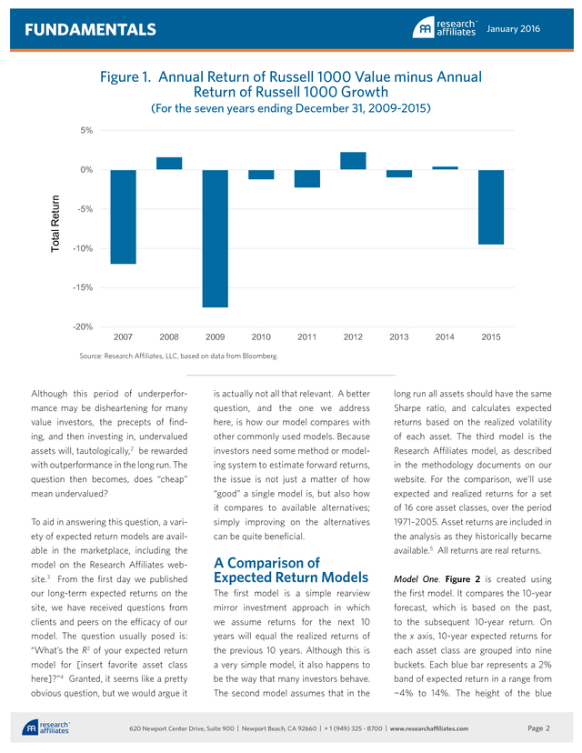
If the cash flows and discount rate remain constant over the holding period, the asset’s value will remain the same throughout its life as on the day it was purchased. Therefore, it is a rate that ultimately drives an asset’s realized return over time, and the possibility of such changes that drives an asset’s expected return over time. As mentioned in the introduction, the implementer of a value strategy would have experienced a long string of annual negative returns over the past several years. Figure 1 illustrates quite vividly the disappointing returns associated with a U.S.
equity value strategy compared with a U.S. equity growth strategy since 2007. Media Contacts United States and Canada Hewes Communications + 1 (212) 207-9450 hewesteam@hewescomm.com Europe JPES Partners (London) +44 (0) 20 7520 7620 ra@jpespartners.com . FUNDAMENTALS January 2016 Figure 1. Annual Return of Russell 1000 Value minus Annual Return of Russell 1000 Growth (For the seven years ending December 31, 2009-2015) 5% Total Return 0% -5% -10% -15% -20% 2007 2008 2009 2010 2011 2012 2013 2014 2015 Source: Research Affiliates, LLC, based on data from Bloomberg. Although this period of underperformance may be disheartening for many value investors, the precepts of finding, and then investing in, undervalued assets will, tautologically,2 be rewarded with outperformance in the long run. The question then becomes, does “cheap” mean undervalued? To aid in answering this question, a variety of expected return models are available in the marketplace, including the model on the Research Affiliates website.3 From the first day we published our long-term expected returns on the site, we have received questions from clients and peers on the efficacy of our model. The question usually posed is: “What’s the R2 of your expected return model for [insert favorite asset class here]?”4 Granted, it seems like a pretty obvious question, but we would argue it is actually not all that relevant.
A better question, and the one we address here, is how our model compares with other commonly used models. Because investors need some method or modeling system to estimate forward returns, the issue is not just a matter of how “good” a single model is, but also how it compares to available alternatives; simply improving on the alternatives can be quite beneficial. A Comparison of Expected Return Models The first model is a simple rearview mirror investment approach in which we assume returns for the next 10 years will equal the realized returns of the previous 10 years. Although this is a very simple model, it also happens to be the way that many investors behave. The second model assumes that in the long run all assets should have the same Sharpe ratio, and calculates expected returns based on the realized volatility of each asset.
The third model is the Research Affiliates model, as described in the methodology documents on our website. For the comparison, we’ll use expected and realized returns for a set of 16 core asset classes, over the period 1971–2005. Asset returns are included in the analysis as they historically became available.5 All returns are real returns. Model One.
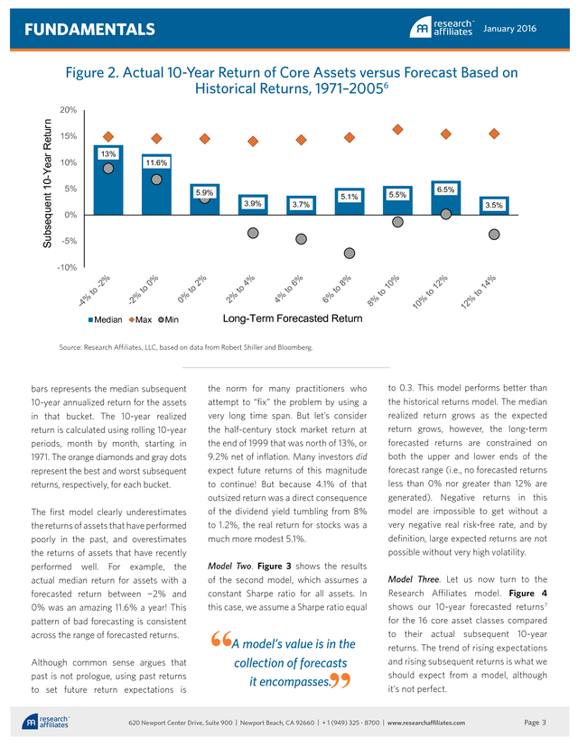
Figure 2 is created using the first model. It compares the 10-year forecast, which is based on the past, to the subsequent 10-year return. On the x axis, 10-year expected returns for each asset class are grouped into nine buckets.
Each blue bar represents a 2% band of expected return in a range from −4% to 14%. The height of the blue 620 Newport Center Drive, Suite 900 | Newport Beach, CA 92660 | + 1 (949) 325 - 8700 | www.researchaffiliates.com Page 2 . FUNDAMENTALS January 2016 Figure 2. Actual 10-Year Return of Core Assets versus Forecast Based on Historical Returns, 1971–20056 Subsequent 10-Year Return 20% 15% 10% 13% 11.6% 5% 5.9% 3.9% 0% 3.7% 5.1% 5.5% 6.5% 3.5% -5% -10% Median Max Min Long-Term Forecasted Return Source: Research Affiliates, LLC, based on data from Robert Shiller and Bloomberg. The first model clearly underestimates the returns of assets that have performed poorly in the past, and overestimates the returns of assets that have recently performed well. For example, the actual median return for assets with a forecasted return between −2% and 0% was an amazing 11.6% a year! This pattern of bad forecasting is consistent across the range of forecasted returns. Although common sense argues that past is not prologue, using past returns to set future return expectations is the norm for many practitioners who attempt to “fix” the problem by using a very long time span. But let’s consider the half-century stock market return at the end of 1999 that was north of 13%, or 9.2% net of inflation.
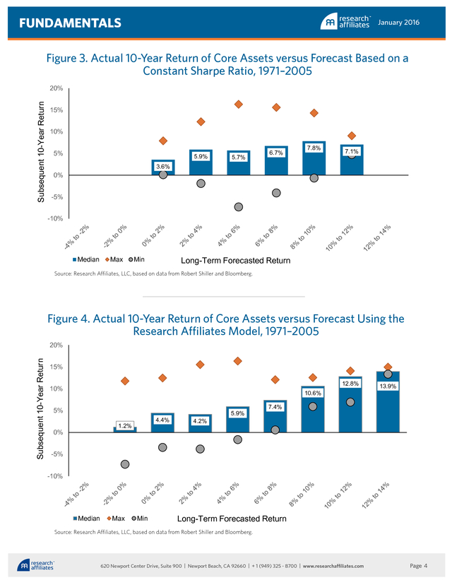
Many investors did expect future returns of this magnitude to continue! But because 4.1% of that outsized return was a direct consequence of the dividend yield tumbling from 8% to 1.2%, the real return for stocks was a much more modest 5.1%. Model Two. Figure 3 shows the results of the second model, which assumes a constant Sharpe ratio for all assets. In this case, we assume a Sharpe ratio equal “ A model’s value is in the collection of forecasts it encompasses. “ bars represents the median subsequent 10-year annualized return for the assets in that bucket.
The 10-year realized return is calculated using rolling 10-year periods, month by month, starting in 1971. The orange diamonds and gray dots represent the best and worst subsequent returns, respectively, for each bucket. to 0.3. This model performs better than the historical returns model.
The median realized return grows as the expected return grows, however, the long-term forecasted returns are constrained on both the upper and lower ends of the forecast range (i.e., no forecasted returns less than 0% nor greater than 12% are generated). Negative returns in this model are impossible to get without a very negative real risk-free rate, and by definition, large expected returns are not possible without very high volatility. Model Three. Let us now turn to the Research Affiliates model.
Figure 4 shows our 10-year forecasted returns7 for the 16 core asset classes compared to their actual subsequent 10-year returns. The trend of rising expectations and rising subsequent returns is what we should expect from a model, although it’s not perfect. 620 Newport Center Drive, Suite 900 | Newport Beach, CA 92660 | + 1 (949) 325 - 8700 | www.researchaffiliates.com Page 3 . FUNDAMENTALS January 2016 Figure 3. Actual 10-Year Return of Core Assets versus Forecast Based on a Constant Sharpe Ratio, 1971–2005 Subsequent 10-Year Return 20% 15% 10% 5% 5.9% 5.7% 6.7% 7.8% 7.1% 3.6% 0% -5% -10% Median Max Long-Term Forecasted Return Min Source: Research Affiliates, LLC, based on data from Robert Shiller and Bloomberg. Figure 4. Actual 10-Year Return of Core Assets versus Forecast Using the Research Affiliates Model, 1971–2005 Subsequent 10-Year Return 20% 15% 12.8% 10% 10.6% 5% 4.4% 1.2% 0% 4.2% 5.9% 13.9% 7.4% -5% -10% Median Max Min Long-Term Forecasted Return Source: Research Affiliates, LLC, based on data from Robert Shiller and Bloomberg. 620 Newport Center Drive, Suite 900 | Newport Beach, CA 92660 | + 1 (949) 325 - 8700 | www.researchaffiliates.com Page 4 . FUNDAMENTALS January 2016 As Figure 4 shows, when our return expectations have been less than 2%, realized returns have often been higher than expected. Although we were apparently overly bearish, our return forecasts were well within the bounds of best and worst realized returns. It is also worth mentioning that market valuation levels have been generally rising, and yields falling, since 1971, so it is possible that our forecasts were correct, net of the (very long) secular trend in valuation levels. belief that the largest and most loss of capital,8 which happens when persistent active investment opportunity investors succumb to fearful thoughts is and thus sell at inopportune times, is long-horizon mean reversion. Investing using a yield-based signal does not come without its challenges. One big challenge is that a yield signal is a valuation signal that does not come with a timing signal. Because the yield is signaling an asset is attractive today does not mean it will not continue to get more attractive.
If the asset’s price falls further, increasing the long-term return outlook, unrealized losses in the For forecasted returns higher than 2%, the median return for each bucket is in line with expectations, with the gap between the minimum and maximum returns becoming smaller as the expected return gets larger. portfolio can be uncomfortable. This It’s important to recognize our expected returns are based on yield, a contrarian signal which echoes our investment discomfort is not due to dollars actually lost, but by the sickening feeling that accompanies downside volatility. As the investor’s true risk. Putting It All Together The primary purpose of an expected return model is to classify what we know about assets in an economically intuitive framework for the purpose of building portfolios.
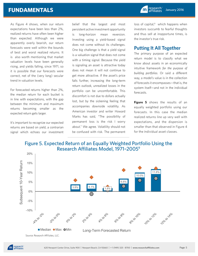
Or said a different way, a model’s value is in the collection of forecasts it encompasses—that is, the system itself—and not in the individual forecasts. Figure 5 shows the results of an equally weighted portfolio using our American investor and writer Howard forecasts. In this case the median Marks has said, “The possibility of realized returns line up very well with permanent loss is the risk I worry expectations, and the dispersion is about.” We agree. Volatility should not smaller than that observed in Figure 4 be confused with risk.
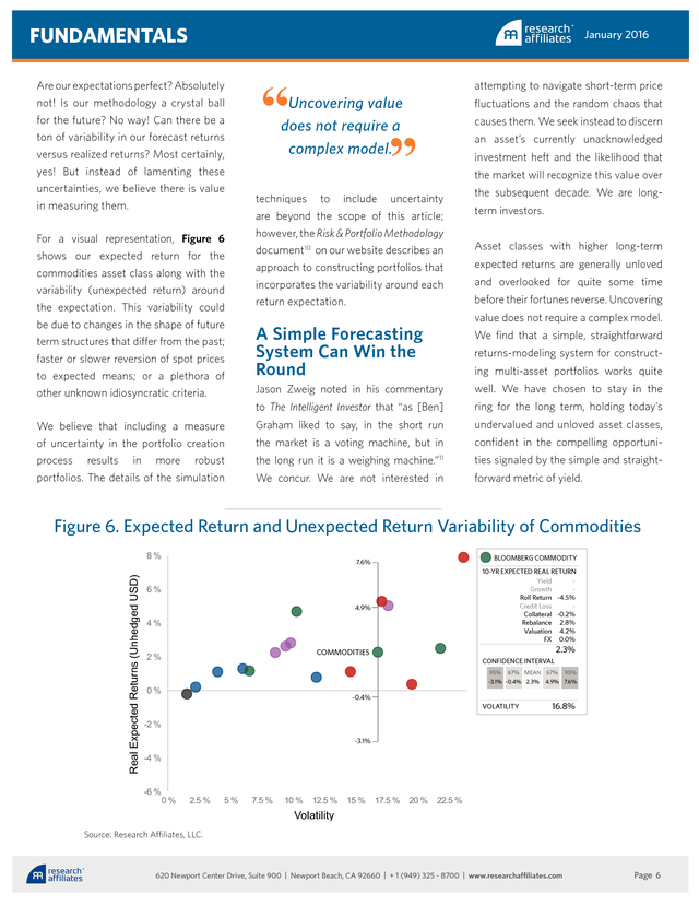
The permanent for the individual asset classes. Figure 5. Expected Return of an Equally Weighted Portfolio Using the Research Affiliates Model, 1971–20059 Subsequent 10-Year Return 20% 15% 10% 10.0% 11.8% 6.8% 5% 3.8% 0% 4.1% 1.8% -5% -10% Median Max Min Long-Term Forecasted Return Source: Research Affiliates, LLC. 620 Newport Center Drive, Suite 900 | Newport Beach, CA 92660 | + 1 (949) 325 - 8700 | www.researchaffiliates.com Page 5 . FUNDAMENTALS January 2016 For a visual representation, Figure 6 shows our expected return for the commodities asset class along with the variability (unexpected return) around the expectation. This variability could be due to changes in the shape of future term structures that differ from the past; faster or slower reversion of spot prices to expected means; or a plethora of other unknown idiosyncratic criteria. We believe that including a measure of uncertainty in the portfolio creation process results in more robust portfolios. The details of the simulation “ attempting to navigate short-term price Uncovering value does not require a complex model. fluctuations and the random chaos that “ Are our expectations perfect? Absolutely not! Is our methodology a crystal ball for the future? No way! Can there be a ton of variability in our forecast returns versus realized returns? Most certainly, yes! But instead of lamenting these uncertainties, we believe there is value in measuring them. causes them. We seek instead to discern an asset’s currently unacknowledged investment heft and the likelihood that the market will recognize this value over techniques to include uncertainty are beyond the scope of this article; however, the Risk & Portfolio Methodology document10 on our website describes an approach to constructing portfolios that incorporates the variability around each return expectation. the subsequent decade.
We are longterm investors. Asset classes with higher long-term expected returns are generally unloved and overlooked for quite some time before their fortunes reverse. Uncovering value does not require a complex model. A Simple Forecasting System Can Win the Round We find that a simple, straightforward returns-modeling system for constructing multi-asset portfolios works quite Jason Zweig noted in his commentary well. We have chosen to stay in the to The Intelligent Investor that “as [Ben] ring for the long term, holding today’s Graham liked to say, in the short run undervalued and unloved asset classes, the market is a voting machine, but in confident in the compelling opportuni- the long run it is a weighing machine.” ties signaled by the simple and straight- We concur.
We are not interested in forward metric of yield. 11 Figure 6. Expected Return and Unexpected Return Variability of Commodities Real Expected Returns (Unhedged USD) 8% BLOOMBERG COMMODITY 7.6% 10-YR EXPECTED REAL RETURN Yield Growth Roll Return -4.5% Credit Loss Collateral -0.2% Rebalance 2.8% Valuation 4.2% FX 0.0% 6% 4.9% 4% 2.3% COMMODITIES 2% CONFIDENCE INTERVAL 95% 67% MEAN 67% 95% -3.1% -0.4% 2.3% 4.9% 7.6% 0% -0.4% VOLATILITY 16.8% -2 % -3.1% -4 % -6 % 0% 2.5 % 5% 7.5 % 10 % 12.5 % 15 % 17.5 % 20 % 22.5 % Volatility Source: Research Affiliates, LLC. 620 Newport Center Drive, Suite 900 | Newport Beach, CA 92660 | + 1 (949) 325 - 8700 | www.researchaffiliates.com Page 6 . FUNDAMENTALS Endnotes 6. 1. Poincaré (1913, p. 10). 2. If it fails to eventually outperform, it’s not undervalued! 3. http:/ /www.researchaffiliates.com/assetallocation. 4. Although measuring the R2 of our models is possible, the result is not very useful because samples overlap over long-term horizons. Take U.S. equities for which data are readily available since the late 1800s, roughly 150 years. We analyze 10-year returns, calculated monthly.
As a result, we have only 15 unique samples. Any regression using monthly data points for 10-year returns will show misrepresented R2 values, because each data point shares 119 of its 120 months with the next data point. Going to non-overlapping returns means we don’t have enough samples for robust results. For example, imagine the same test for the Barclays U.S.
Aggregate Bond Index, which started in 1976—four samples anyone? 5. January 2016 Indices were added as data became available: 8/1971, Russell 2000; 12/1988, MSCI EAFE; 1/1990, Barclays Corporate High Yield; 1/1992, Barclays U.S. Treasury Long; 5/1992, Barclays U.S. Aggregate; 5/1992, JPMorgan EMBI+ (Hard Currency); 4/1994, Barclays U.S.
Treasury 1–3yr; 1/1997, Bloomberg Commodity Index; 3/1997, JPMorgan ELMI+; 1/2001, Barclays U.S. Treasury TIPS; 7/2003, FTSE NAREIT. Analysis is monthly and ends in 2005, the most recent date for which 10-year subsequent returns can be calculated. The range for each of the bars in the chart should be interpreted as including the lower bound but not the upper bound of the range.
For example, the range −2% to 0% includes returns from, and including, −2% up to, but not including, 0%. This standard also applies to the charts in Figures 3–5. 7. These forecasted returns represent return expectations that our methodology would have delivered in past decades. The core elements of the methodology were first described by Arnott and Von Germeten (1983); thus, the methodology is not a data-mining exercise of fitting past market returns. 8. Marks (2013, p.
45). 9. The 4% to 6% bucket is an outlier here; however, this result only occurred in 13 months of the entire 34-year period. 10. http://www.researchaffiliates.com/Production%20content%20library/ AA-Asset-Class-Risk.pdf?print=1. 11. Graham (2006, p. 477) . References Arnott, Robert, and James Von Germeten. 1983.
“Systematic Asset Allocation.” Financial Analysts Journal, vol. 39, no. 6 (November/December): 31–38. Graham, Benjamin.
2006 (1973). The Intelligent Investor—Fourth Revised Edition, with new commentary by Jason Zweig. New York: HarperCollins Publisher. Marks, Howard.
2013. The Most Important Thing Illuminated. New York: Columbia University Press. Poincaré, Henri.
1913. The Foundations of Science. New York City and Garrison, NY: The Science Press. Disclosures The material contained in this document is for general information purposes only.
It is not intended as an offer or a solicitation for the purchase and/or sale of any security, derivative, commodity, or financial instrument, nor is it advice or a recommendation to enter into any transaction. Research results relate only to a hypothetical model of past performance (i.e., a simulation) and not to an asset management product. No allowance has been made for trading costs or management fees, which would reduce investment performance.
Actual results may differ. Index returns represent back-tested performance based on rules used in the creation of the index, are not a guarantee of future performance, and are not indicative of any specific investment. Indexes are not managed investment products and cannot be invested in directly.
This material is based on information that is considered to be reliable, but Research Affiliates™ and its related entities (collectively “Research Affiliates”) make this information available on an “as is” basis without a duty to update, make warranties, express or implied, regarding the accuracy of the information contained herein. Research Affiliates is not responsible for any errors or omissions or for results obtained from the use of this information. Nothing contained in this material is intended to constitute legal, tax, securities, financial or investment advice, nor an opinion regarding the appropriateness of any investment.
The information contained in this material should not be acted upon without obtaining advice from a licensed professional. Research Affiliates, LLC, is an investment adviser registered under the Investment Advisors Act of 1940 with the U.S. Securities and Exchange Commission (SEC).
Our registration as an investment adviser does not imply a certain level of skill or training. Investors should be aware of the risks associated with data sources and quantitative processes used in our investment management process. Errors may exist in data acquired from third party vendors, the construction of model portfolios, and in coding related to the index and portfolio construction process. While Research Affiliates takes steps to identify data and process errors so as to minimize the potential impact of such errors on index and portfolio performance, we cannot guarantee that such errors will not occur. The trademarks Fundamental Index™, RAFI™, Research Affiliates Equity™, RAE™, and the Research Affiliates™ trademark and corporate name and all related logos are the exclusive intellectual property of Research Affiliates, LLC and in some cases are registered trademarks in the U.S. and other countries. Various features of the Fundamental Index™ methodology, including an accounting data-based non-capitalization data processing system and method for creating and weighting an index of securities, are protected by various patents, and patent-pending intellectual property of Research Affiliates, LLC.
(See all applicable US Patents, Patent Publications, Patent Pending intellectual property and protected trademarks located at http:/ /www.researchaffiliates.com/ Pages/ legal.aspx#d, which are fully incorporated herein.) Any use of these trademarks, logos, patented or patent pending methodologies without the prior written permission of Research Affiliates, LLC, is expressly prohibited. Research Affiliates, LLC, reserves the right to take any and all necessary action to preserve all of its rights, title, and interest in and to these marks, patents or pending patents. The views and opinions expressed are those of the author and not necessarily those of Research Affiliates, LLC. The opinions are subject to change without notice. ©2016 Research Affiliates, LLC.
All rights reserved. 620 Newport Center Drive, Suite 900 | Newport Beach, CA 92660 | + 1 (949) 325 - 8700 | www.researchaffiliates.com Page 7 .
In this article, we compare three models. Each can be classified as simple in contrast to the quite complex models used by many institutional investors. One of the three is the model used by Research Affiliates, which although simple has performed well, not only in terms of making long-term asset class forecasts, but in combining undervalued asset classes to build alpha-generating portfolios.
This latter consideration is a prime attribute of a successful model. change in the cash flows and/or the discount investments we make. Whether an investor practices top-down asset allocation or bottom-up security selection, investing is about nothing more than securing cash flows at a reasonable price. After all, the price of an asset is simply the sum of its discounted cash flows, which can be affected by two forces: 1) changes in the cash flows and/or 2) changes in the discount rate.
If the cash flows and discount rate remain constant over the holding period, the asset’s value will remain the same throughout its life as on the day it was purchased. Therefore, it is a rate that ultimately drives an asset’s realized return over time, and the possibility of such changes that drives an asset’s expected return over time. As mentioned in the introduction, the implementer of a value strategy would have experienced a long string of annual negative returns over the past several years. Figure 1 illustrates quite vividly the disappointing returns associated with a U.S.
equity value strategy compared with a U.S. equity growth strategy since 2007. Media Contacts United States and Canada Hewes Communications + 1 (212) 207-9450 hewesteam@hewescomm.com Europe JPES Partners (London) +44 (0) 20 7520 7620 ra@jpespartners.com . FUNDAMENTALS January 2016 Figure 1. Annual Return of Russell 1000 Value minus Annual Return of Russell 1000 Growth (For the seven years ending December 31, 2009-2015) 5% Total Return 0% -5% -10% -15% -20% 2007 2008 2009 2010 2011 2012 2013 2014 2015 Source: Research Affiliates, LLC, based on data from Bloomberg. Although this period of underperformance may be disheartening for many value investors, the precepts of finding, and then investing in, undervalued assets will, tautologically,2 be rewarded with outperformance in the long run. The question then becomes, does “cheap” mean undervalued? To aid in answering this question, a variety of expected return models are available in the marketplace, including the model on the Research Affiliates website.3 From the first day we published our long-term expected returns on the site, we have received questions from clients and peers on the efficacy of our model. The question usually posed is: “What’s the R2 of your expected return model for [insert favorite asset class here]?”4 Granted, it seems like a pretty obvious question, but we would argue it is actually not all that relevant.
A better question, and the one we address here, is how our model compares with other commonly used models. Because investors need some method or modeling system to estimate forward returns, the issue is not just a matter of how “good” a single model is, but also how it compares to available alternatives; simply improving on the alternatives can be quite beneficial. A Comparison of Expected Return Models The first model is a simple rearview mirror investment approach in which we assume returns for the next 10 years will equal the realized returns of the previous 10 years. Although this is a very simple model, it also happens to be the way that many investors behave. The second model assumes that in the long run all assets should have the same Sharpe ratio, and calculates expected returns based on the realized volatility of each asset.
The third model is the Research Affiliates model, as described in the methodology documents on our website. For the comparison, we’ll use expected and realized returns for a set of 16 core asset classes, over the period 1971–2005. Asset returns are included in the analysis as they historically became available.5 All returns are real returns. Model One.
Figure 2 is created using the first model. It compares the 10-year forecast, which is based on the past, to the subsequent 10-year return. On the x axis, 10-year expected returns for each asset class are grouped into nine buckets.
Each blue bar represents a 2% band of expected return in a range from −4% to 14%. The height of the blue 620 Newport Center Drive, Suite 900 | Newport Beach, CA 92660 | + 1 (949) 325 - 8700 | www.researchaffiliates.com Page 2 . FUNDAMENTALS January 2016 Figure 2. Actual 10-Year Return of Core Assets versus Forecast Based on Historical Returns, 1971–20056 Subsequent 10-Year Return 20% 15% 10% 13% 11.6% 5% 5.9% 3.9% 0% 3.7% 5.1% 5.5% 6.5% 3.5% -5% -10% Median Max Min Long-Term Forecasted Return Source: Research Affiliates, LLC, based on data from Robert Shiller and Bloomberg. The first model clearly underestimates the returns of assets that have performed poorly in the past, and overestimates the returns of assets that have recently performed well. For example, the actual median return for assets with a forecasted return between −2% and 0% was an amazing 11.6% a year! This pattern of bad forecasting is consistent across the range of forecasted returns. Although common sense argues that past is not prologue, using past returns to set future return expectations is the norm for many practitioners who attempt to “fix” the problem by using a very long time span. But let’s consider the half-century stock market return at the end of 1999 that was north of 13%, or 9.2% net of inflation.
Many investors did expect future returns of this magnitude to continue! But because 4.1% of that outsized return was a direct consequence of the dividend yield tumbling from 8% to 1.2%, the real return for stocks was a much more modest 5.1%. Model Two. Figure 3 shows the results of the second model, which assumes a constant Sharpe ratio for all assets. In this case, we assume a Sharpe ratio equal “ A model’s value is in the collection of forecasts it encompasses. “ bars represents the median subsequent 10-year annualized return for the assets in that bucket.
The 10-year realized return is calculated using rolling 10-year periods, month by month, starting in 1971. The orange diamonds and gray dots represent the best and worst subsequent returns, respectively, for each bucket. to 0.3. This model performs better than the historical returns model.
The median realized return grows as the expected return grows, however, the long-term forecasted returns are constrained on both the upper and lower ends of the forecast range (i.e., no forecasted returns less than 0% nor greater than 12% are generated). Negative returns in this model are impossible to get without a very negative real risk-free rate, and by definition, large expected returns are not possible without very high volatility. Model Three. Let us now turn to the Research Affiliates model.
Figure 4 shows our 10-year forecasted returns7 for the 16 core asset classes compared to their actual subsequent 10-year returns. The trend of rising expectations and rising subsequent returns is what we should expect from a model, although it’s not perfect. 620 Newport Center Drive, Suite 900 | Newport Beach, CA 92660 | + 1 (949) 325 - 8700 | www.researchaffiliates.com Page 3 . FUNDAMENTALS January 2016 Figure 3. Actual 10-Year Return of Core Assets versus Forecast Based on a Constant Sharpe Ratio, 1971–2005 Subsequent 10-Year Return 20% 15% 10% 5% 5.9% 5.7% 6.7% 7.8% 7.1% 3.6% 0% -5% -10% Median Max Long-Term Forecasted Return Min Source: Research Affiliates, LLC, based on data from Robert Shiller and Bloomberg. Figure 4. Actual 10-Year Return of Core Assets versus Forecast Using the Research Affiliates Model, 1971–2005 Subsequent 10-Year Return 20% 15% 12.8% 10% 10.6% 5% 4.4% 1.2% 0% 4.2% 5.9% 13.9% 7.4% -5% -10% Median Max Min Long-Term Forecasted Return Source: Research Affiliates, LLC, based on data from Robert Shiller and Bloomberg. 620 Newport Center Drive, Suite 900 | Newport Beach, CA 92660 | + 1 (949) 325 - 8700 | www.researchaffiliates.com Page 4 . FUNDAMENTALS January 2016 As Figure 4 shows, when our return expectations have been less than 2%, realized returns have often been higher than expected. Although we were apparently overly bearish, our return forecasts were well within the bounds of best and worst realized returns. It is also worth mentioning that market valuation levels have been generally rising, and yields falling, since 1971, so it is possible that our forecasts were correct, net of the (very long) secular trend in valuation levels. belief that the largest and most loss of capital,8 which happens when persistent active investment opportunity investors succumb to fearful thoughts is and thus sell at inopportune times, is long-horizon mean reversion. Investing using a yield-based signal does not come without its challenges. One big challenge is that a yield signal is a valuation signal that does not come with a timing signal. Because the yield is signaling an asset is attractive today does not mean it will not continue to get more attractive.
If the asset’s price falls further, increasing the long-term return outlook, unrealized losses in the For forecasted returns higher than 2%, the median return for each bucket is in line with expectations, with the gap between the minimum and maximum returns becoming smaller as the expected return gets larger. portfolio can be uncomfortable. This It’s important to recognize our expected returns are based on yield, a contrarian signal which echoes our investment discomfort is not due to dollars actually lost, but by the sickening feeling that accompanies downside volatility. As the investor’s true risk. Putting It All Together The primary purpose of an expected return model is to classify what we know about assets in an economically intuitive framework for the purpose of building portfolios.
Or said a different way, a model’s value is in the collection of forecasts it encompasses—that is, the system itself—and not in the individual forecasts. Figure 5 shows the results of an equally weighted portfolio using our American investor and writer Howard forecasts. In this case the median Marks has said, “The possibility of realized returns line up very well with permanent loss is the risk I worry expectations, and the dispersion is about.” We agree. Volatility should not smaller than that observed in Figure 4 be confused with risk.
The permanent for the individual asset classes. Figure 5. Expected Return of an Equally Weighted Portfolio Using the Research Affiliates Model, 1971–20059 Subsequent 10-Year Return 20% 15% 10% 10.0% 11.8% 6.8% 5% 3.8% 0% 4.1% 1.8% -5% -10% Median Max Min Long-Term Forecasted Return Source: Research Affiliates, LLC. 620 Newport Center Drive, Suite 900 | Newport Beach, CA 92660 | + 1 (949) 325 - 8700 | www.researchaffiliates.com Page 5 . FUNDAMENTALS January 2016 For a visual representation, Figure 6 shows our expected return for the commodities asset class along with the variability (unexpected return) around the expectation. This variability could be due to changes in the shape of future term structures that differ from the past; faster or slower reversion of spot prices to expected means; or a plethora of other unknown idiosyncratic criteria. We believe that including a measure of uncertainty in the portfolio creation process results in more robust portfolios. The details of the simulation “ attempting to navigate short-term price Uncovering value does not require a complex model. fluctuations and the random chaos that “ Are our expectations perfect? Absolutely not! Is our methodology a crystal ball for the future? No way! Can there be a ton of variability in our forecast returns versus realized returns? Most certainly, yes! But instead of lamenting these uncertainties, we believe there is value in measuring them. causes them. We seek instead to discern an asset’s currently unacknowledged investment heft and the likelihood that the market will recognize this value over techniques to include uncertainty are beyond the scope of this article; however, the Risk & Portfolio Methodology document10 on our website describes an approach to constructing portfolios that incorporates the variability around each return expectation. the subsequent decade.
We are longterm investors. Asset classes with higher long-term expected returns are generally unloved and overlooked for quite some time before their fortunes reverse. Uncovering value does not require a complex model. A Simple Forecasting System Can Win the Round We find that a simple, straightforward returns-modeling system for constructing multi-asset portfolios works quite Jason Zweig noted in his commentary well. We have chosen to stay in the to The Intelligent Investor that “as [Ben] ring for the long term, holding today’s Graham liked to say, in the short run undervalued and unloved asset classes, the market is a voting machine, but in confident in the compelling opportuni- the long run it is a weighing machine.” ties signaled by the simple and straight- We concur.
We are not interested in forward metric of yield. 11 Figure 6. Expected Return and Unexpected Return Variability of Commodities Real Expected Returns (Unhedged USD) 8% BLOOMBERG COMMODITY 7.6% 10-YR EXPECTED REAL RETURN Yield Growth Roll Return -4.5% Credit Loss Collateral -0.2% Rebalance 2.8% Valuation 4.2% FX 0.0% 6% 4.9% 4% 2.3% COMMODITIES 2% CONFIDENCE INTERVAL 95% 67% MEAN 67% 95% -3.1% -0.4% 2.3% 4.9% 7.6% 0% -0.4% VOLATILITY 16.8% -2 % -3.1% -4 % -6 % 0% 2.5 % 5% 7.5 % 10 % 12.5 % 15 % 17.5 % 20 % 22.5 % Volatility Source: Research Affiliates, LLC. 620 Newport Center Drive, Suite 900 | Newport Beach, CA 92660 | + 1 (949) 325 - 8700 | www.researchaffiliates.com Page 6 . FUNDAMENTALS Endnotes 6. 1. Poincaré (1913, p. 10). 2. If it fails to eventually outperform, it’s not undervalued! 3. http:/ /www.researchaffiliates.com/assetallocation. 4. Although measuring the R2 of our models is possible, the result is not very useful because samples overlap over long-term horizons. Take U.S. equities for which data are readily available since the late 1800s, roughly 150 years. We analyze 10-year returns, calculated monthly.
As a result, we have only 15 unique samples. Any regression using monthly data points for 10-year returns will show misrepresented R2 values, because each data point shares 119 of its 120 months with the next data point. Going to non-overlapping returns means we don’t have enough samples for robust results. For example, imagine the same test for the Barclays U.S.
Aggregate Bond Index, which started in 1976—four samples anyone? 5. January 2016 Indices were added as data became available: 8/1971, Russell 2000; 12/1988, MSCI EAFE; 1/1990, Barclays Corporate High Yield; 1/1992, Barclays U.S. Treasury Long; 5/1992, Barclays U.S. Aggregate; 5/1992, JPMorgan EMBI+ (Hard Currency); 4/1994, Barclays U.S.
Treasury 1–3yr; 1/1997, Bloomberg Commodity Index; 3/1997, JPMorgan ELMI+; 1/2001, Barclays U.S. Treasury TIPS; 7/2003, FTSE NAREIT. Analysis is monthly and ends in 2005, the most recent date for which 10-year subsequent returns can be calculated. The range for each of the bars in the chart should be interpreted as including the lower bound but not the upper bound of the range.
For example, the range −2% to 0% includes returns from, and including, −2% up to, but not including, 0%. This standard also applies to the charts in Figures 3–5. 7. These forecasted returns represent return expectations that our methodology would have delivered in past decades. The core elements of the methodology were first described by Arnott and Von Germeten (1983); thus, the methodology is not a data-mining exercise of fitting past market returns. 8. Marks (2013, p.
45). 9. The 4% to 6% bucket is an outlier here; however, this result only occurred in 13 months of the entire 34-year period. 10. http://www.researchaffiliates.com/Production%20content%20library/ AA-Asset-Class-Risk.pdf?print=1. 11. Graham (2006, p. 477) . References Arnott, Robert, and James Von Germeten. 1983.
“Systematic Asset Allocation.” Financial Analysts Journal, vol. 39, no. 6 (November/December): 31–38. Graham, Benjamin.
2006 (1973). The Intelligent Investor—Fourth Revised Edition, with new commentary by Jason Zweig. New York: HarperCollins Publisher. Marks, Howard.
2013. The Most Important Thing Illuminated. New York: Columbia University Press. Poincaré, Henri.
1913. The Foundations of Science. New York City and Garrison, NY: The Science Press. Disclosures The material contained in this document is for general information purposes only.
It is not intended as an offer or a solicitation for the purchase and/or sale of any security, derivative, commodity, or financial instrument, nor is it advice or a recommendation to enter into any transaction. Research results relate only to a hypothetical model of past performance (i.e., a simulation) and not to an asset management product. No allowance has been made for trading costs or management fees, which would reduce investment performance.
Actual results may differ. Index returns represent back-tested performance based on rules used in the creation of the index, are not a guarantee of future performance, and are not indicative of any specific investment. Indexes are not managed investment products and cannot be invested in directly.
This material is based on information that is considered to be reliable, but Research Affiliates™ and its related entities (collectively “Research Affiliates”) make this information available on an “as is” basis without a duty to update, make warranties, express or implied, regarding the accuracy of the information contained herein. Research Affiliates is not responsible for any errors or omissions or for results obtained from the use of this information. Nothing contained in this material is intended to constitute legal, tax, securities, financial or investment advice, nor an opinion regarding the appropriateness of any investment.
The information contained in this material should not be acted upon without obtaining advice from a licensed professional. Research Affiliates, LLC, is an investment adviser registered under the Investment Advisors Act of 1940 with the U.S. Securities and Exchange Commission (SEC).
Our registration as an investment adviser does not imply a certain level of skill or training. Investors should be aware of the risks associated with data sources and quantitative processes used in our investment management process. Errors may exist in data acquired from third party vendors, the construction of model portfolios, and in coding related to the index and portfolio construction process. While Research Affiliates takes steps to identify data and process errors so as to minimize the potential impact of such errors on index and portfolio performance, we cannot guarantee that such errors will not occur. The trademarks Fundamental Index™, RAFI™, Research Affiliates Equity™, RAE™, and the Research Affiliates™ trademark and corporate name and all related logos are the exclusive intellectual property of Research Affiliates, LLC and in some cases are registered trademarks in the U.S. and other countries. Various features of the Fundamental Index™ methodology, including an accounting data-based non-capitalization data processing system and method for creating and weighting an index of securities, are protected by various patents, and patent-pending intellectual property of Research Affiliates, LLC.
(See all applicable US Patents, Patent Publications, Patent Pending intellectual property and protected trademarks located at http:/ /www.researchaffiliates.com/ Pages/ legal.aspx#d, which are fully incorporated herein.) Any use of these trademarks, logos, patented or patent pending methodologies without the prior written permission of Research Affiliates, LLC, is expressly prohibited. Research Affiliates, LLC, reserves the right to take any and all necessary action to preserve all of its rights, title, and interest in and to these marks, patents or pending patents. The views and opinions expressed are those of the author and not necessarily those of Research Affiliates, LLC. The opinions are subject to change without notice. ©2016 Research Affiliates, LLC.
All rights reserved. 620 Newport Center Drive, Suite 900 | Newport Beach, CA 92660 | + 1 (949) 325 - 8700 | www.researchaffiliates.com Page 7 .


