


Description
Default Probability and Loss Given Default
for Home Equity Loans
Michael LaCour-Little
Yanan Zhang
Office of the Comptroller of the Currency
Economics Working Paper 2014-1
June 2014
Keywords: mortgage default, loss given default, home equity loans, securitization.
JEL classifications: G21, G28.
Michael LaCour-Little is a professor of finance at California State University at Fullerton (e-mail
mlacour-little@fullerton.edu). Yanan Zhang is a financial economist at the Office of the
Comptroller of the Currency (e-mail yanan.zhang@occ.treas.gov), 400 7th St. SW, Washington,
DC 20219, telephone (202) 649-5465; fax (571) 465-3935.
The views expressed in this paper are those of the authors alone and do not necessarily reflect
those of the Office of the Comptroller of the Currency or the U.S. Department of the Treasury.
The authors would like to thank Michele Tezduyar for editorial assistance.
The authors take responsibility for any errors. . Default Probability and Loss Given Default for Home Equity Loans Michael LaCour-Little Yanan Zhang June 2014 Abstract: Securitization has been widely assigned blame for contributing to the recent mortgage market meltdown and ensuing financial crisis. In this paper, we sample from the OCC Mortgage Metrics database to develop estimates of default probabilities and loss given default for home equity loans originated during 2004-2008 and tracked from 2008-2012. We are particularly interested in the relationship between loan outcomes and the lender’s decision to securitize the asset. Among other innovations, we are able to measure the change in the borrower’s credit score over time and the level of documentation used during loan underwriting.
Results suggest that securitized home equity loans bear higher default risk and produce greater loss severity than loans held in portfolio by lenders. Economics Working Paper 2014-1 i . 1. Introduction Securitization, particularly non-agency securitization of subprime and Alt-A mortgages, has been identified as a contributory factor in the recent financial crisis (see, for example, Keys, Mukherjee, Seru, and Vig [2010] or Keys, Seru, and Vig [2012]). While first mortgage loans have been widely studied, home equity loans have not. The current paper addresses this gap in the literature utilizing the Office of the Comptroller of the Currency (OCC) Mortgage Metrics dataset.
To preview our main result, we find that securitized home equity loans do have greater default probability (PD) and loss given default (LGD) than loans retained in portfolio by major banks. While less frequently studied than first mortgages, home equity loans grew rapidly during the period 2000-2008 and became a sizable segment of the mortgage market. The total dollars outstanding of home equity loans increased from $275.5 billion in 2000 to a peak of $953.5 billion in 2008, an average annual growth rate of 16.8 percent. Likewise, the total number of home equity loans increased from 12.9 million in 2000 to a peak of 23.8 million in 2007, an average annual growth rate of 9.1 percent.
Since balances were growing faster than accounts, average loan size was increasing over the period as well. Unlike first lien loans, the majority of which are securitized, most home equity loans remain on bank balance sheets. Aggregate bank risk exposure to home equity loans is estimated to be 30 percent of the total residential mortgage exposure, or roughly $750 billion (Fitch Ratings, 2012).
As the private-label mortgage securitization market has recently shown signs of resurgence, home equity loans are again evident (Inside Mortgage Finance, 2013). Research has also shown that junior lien lending through home equity loans is related to the documented increase in household leverage (Mian and Sufi [2011]) and to the much-reported decline in personal savings (Greenspan and Kennedy [2008]). Moreover, increased debt usage through home equity lending can also dilute equity in a borrower’s home, thereby increasing the default risk of first mortgages and magnifying the impact of declining house prices on default and foreclosure rates (LaCour-Little [2004]). Likewise, LaCour-Little, Sun, and Yu (2013) find Economics Working Paper 2014-1 1 .
that greater home equity lending at the zip code level, especially of home equity lines of credit (HELOC), is related to higher rates of mortgage default on first mortgages in the same area. Our contribution in this paper is to examine the PD and loss severity of home equity loans during the recent market downturn, 2008-2012. Among other enhancements, we have a measure of borrower credit score over time, allowing us a rough proxy for changes in the borrower’s financial position prior to default. Moreover, we have measures of income and asset verification, so that we can quantify the role of reduced documentation in default risk. The paper is organized as follows. In the next section, we review the literature on mortgage loan performance, and the more limited research on LGD generally and home equity lending in particular.
In the third section, we describe our data and sampling approach. In Section IV, we present regression models of PD and discuss results. Section V presents the data used and regression models estimated for LGD estimates, including a discussion of results.
Section VI presents conclusions and extensions in progress. 2. Literature Review PD and LGD on fixed income instruments are a longstanding topic of interest in finance. For example, Altman, Resti, and Sironi (2003) present a broad review of the literature and the empirical evidence of default recovery rates in credit-risk modeling.
Their paper focuses on the relationship between PD and LGD and how this relationship is treated in different modeling frameworks. Recent empirical evidence cited suggests that LGD is positively correlated with PD. 1 The evolving Basel standards have stimulated additional research on LGD.
Schuermann (2004), for example, analyzes the definition and measurement of LGD in the context of Basel II and analyzes data from Moody’s Default Risk Service Database. Among his findings, he reports that 1 See details of the empirical evidence in Frye (2000a, b), Jarrow (2001), Carey and Gordy (2003), and Altman et al. (2001, 2004). Economics Working Paper 2014-1 2 . the recovery distribution is bimodal, lower in recessions than in expansions. Both the Altman and Schuermann papers are based on corporate bond data. Relatively fewer papers focus on consumer loans, such as credit card or home mortgage debt, although this literature is growing rapidly. This is probably due to the absence of publicly available data, since most of these loans reside on bank balance sheets, and lender focus on PD modeling. An early paper that is focused on LGD for residential mortgages is Lekkas et al. (1993).
They test the frictionless options-based mortgage default theory empirically and report that higher loss severity is associated with higher original loan-to-value (LTV), geographical locations with higher default rates, and younger mortgage loans. Crawford and Rosenblatt (1995) incorporate transaction costs into the options-based mortgage default model and empirically test its effect on loss severity. Among their findings is that LGD is reduced where the probability of a deficiency judgment is higher.
Among more recent papers focused on mortgage loans, Calem and LaCour-Little (2004) also analyze the determinants of LGD. Their regression results confirm Lekkas et al. (1993) for either original LTV or combined loan-to-value (CLTV).
They also report that both mortgage age and loan size have significant effects on LGD, with smaller loans exhibiting higher loss severity due to fixed costs associated with exercising the foreclosure option. More recently, Qi and Yang (2009) study LGD of high LTV loans using data from private mortgage insurance companies. They find that CLTV is the single most important determinant of LGD. They find that mortgage loss severity in distressed housing markets is significantly higher than under normal housing market conditions.
In a study unrelated to mortgage lending, Bellotti and Crook (2009) study LGD models for UK retail credit cards. They compare several econometric methods for modeling LGD and find that Ordinary Least Squares models with macroeconomic variables perform best to forecast LGD at both the account level and the portfolio level. The inclusion of macroeconomic variables enables them to model LGD in downturn conditions as required by Basel II. Most of these studies have focused on testing particular theories and underlying relationships. Studies on business cycle effects remain limited, although there have been some attempts to test Economics Working Paper 2014-1 3 .
the downturn effect. For example, Calem and LaCour-Little (2004) examine the relationship between LGD and the economic environment using simulation at the portfolio level. Qi and Yang (2009), cited above, test the effect of housing market downturns by inclusion of a dummy variable. For home equity lending specifically, the literature is much more limited. Canner, Fergus, and Luckett (1988) describe the early stages and growth of the home equity lending segment, following passage of the 1986 tax law changes which are generally acknowledged to have accelerated the growth of this segment of consumer lending.
2 Weicher (1997) reviews the home equity lending industry during the 1990s, characterizing it as business based on recapitalizing borrowers with impaired credit but substantial housing equity. LaCour-Little, Calhoun, and Yu (2011) focus on simultaneous close or “piggyback” loans, and find that such lending is associated with higher default and foreclosure rates in subsequent years. Goodman, Ashworth, Landy, and Yin (2010) report that the presence of junior lien mortgages increases the default risk of first lien mortgages.
Ambrose, Agrawal, and Liu (2005) show that patterns of home equity line use are also related to borrower credit quality, as measured by their FICO scores. Extending that analysis further, Agarwal, Ambrose, Chomsisengphet, and Liu (2006) examine the performance of home equity lines and loans, finding considerable difference in terms of default and prepayment risk. Agarwal, Ambrose, Chomsisengphet, and Liu (2010) examine the role of soft information in home equity lending and find that its use can be effective in reducing default risk.
LaCour-Little, Rosenblatt, and Yao (2010) document the magnitude of equity extraction by homeowners during the period 2000-2006. Cooper (2010) finds that high equity extraction has been used both for household expenditures and home improvement during the 2000-2006 housing boom. The present paper contributes to the existing literature on LGD and home equity lending in the following ways. First, we sample from a comprehensive dataset of mortgage lending by the largest commercial banks in the U.S.
Second, due to the richness of this dataset, we are able to employ a reasonable proxy for the financial positions of households utilizing their current credit 2 Prior to 1986, most interest on consumer debt was tax-deductible; after the 1986 tax law changes, only residential mortgage debt remained generally deductible for those who itemize deductions. Economics Working Paper 2014-1 4 . scores. Third, we have measures for the level of documentation used in loan underwriting, allowing us to quantify the effect of “low doc” underwriting on default risk. Finally, since we have information on whether the loan was securitized or not, we are able to examine the correlates of that decision on subsequent loan performance. 3. Data and Sampling Scheme The data used in this research is a sample taken from the OCC’s Mortgage Metrics database. This is a loan-level dataset of monthly servicing information from nine large national banks assembled by LPS Applied Analytics and provided to the OCC.
The database is quite rich and contains more than 80 fields. Variables denote the borrower’s credit profile, loan product details, collateral information, and loan performance history, including both delinquency and loan modification information. Collection of monthly performance information began in May 2008 and continues to the present; accordingly, we will be able to update results as more time passes. The underlying loans account for two-thirds of the overall home equity market, and there are more than 9 million loan records added to the database each month.
This is truly “big data.” In table 1A, we present a snapshot of the database as of December 2009 to better illustrate the distribution of loans in the database. There are 10.5 million loans in active status at the end of 2009; of these, 8.2 million are in second lien position; of these, 7.2 million were originated between 2004 and 2008 and are either held in portfolio or securitized by private issuers. Of the 7.2 million second liens, 2.0 million, or about 28 percent, are home equity loans (sometimes called closed end seconds or CES), and the rest are HELOCs. Economics Working Paper 2014-1 5 .
LOAN_OWNER All LoanCount Avg Balance INTRATE_ INTRATE_C CLTV_ CLTV_C FICO_O FICO_C ORIG URR ORIG URR RIG URR DTI arm Income Asset Document Document ed ed subprime All 7,215,037 $56,001 7.29% 5.14% 78.6 74.7 735 717 36.6 73.5% 6.6% 25.3% 11.8% Securitized 542,302 $46,579 7.20% 7.54% 86.2 97.9 715 685 35.7 66.6% 3.0% 39.0% 3.5% Portfolio 6,672,735 $56,762 7.30% 4.94% 78.0 72.8 736 720 36.6 74.1% 6.9% 24.2% 12.5% HE Loan All 2,005,284 $48,522 8.17% 8.00% 84.3 86.9 724 702 36.6 5.7% 14.6% 40.7% 17.3% %Sec'tzd Securitized 182,282 $43,077 8.42% 8.60% 89.2 88.3 713 678 37.3 0.5% 7.8% 48.8% 7.8% Portfolio 1,823,002 $49,057 8.15% 7.94% 83.9 86.7 725 704 36.5 6.2% 15.2% 39.9% 18.3% %Sec'tzd 7.5% 9.1% HELOC %Sec'tzd 6.9% All 5,209,753 $58,870 6.91% 4.03% 76.5 70.6 739 723 36.5 99.7% 3.6% 19.4% 9.7% Securitized 360,020 $48,319 6.62% 7.01% 84.8 102.4 716 689 35.0 100.0% 0.6% 34.0% 1.3% Portfolio 4,849,733 $59,653 6.93% 3.81% 75.8 68.1 741 726 36.7 3.8% 18.3% 10.3% 99.6% The share of securitized loans overall is 7.5 percent. The next table shows how securitization patterns and average loan characteristics have evolved over time. LoanCount AvgBal INTRATE_ INTRATE_ CLTV_ CLTV_C FICO_ FICO_C CURR ORIG ORIG URR ORIG URR origyr securitized DTI arm subprime Doc_i Doc_a 2003 No 533,121 $39,113 5.10% 4.29% 75 51 739 744 32 83% 4% 20% 14% 2003 Yes 42,896 $24,719 4.35% 5.34% 82 72 725 716 32 89% 1% 45% 1% 2004 No 812,061 $47,084 5.40% 4.26% 77 60 737 733 35 86% 6% 22% 15% 2004 Yes 71,001 $35,997 4.83% 6.02% 85 93 719 698 35 94% 5% 46% 9% 2005 No 1,323,251 $55,931 6.87% 4.64% 79 72 735 723 36 78% 9% 24% 14% 2005 Yes 107,594 $45,482 6.38% 7.54% 86 106 715 680 35 91% 8% 43% 8% 2006 No 1,628,302 $61,651 8.20% 5.27% 79 77 733 709 38 68% 10% 21% 11% 2006 Yes 208,498 $52,215 8.27% 8.17% 87 96 711 676 37 52% 2% 35% 2% 2007 No 1,793,137 $61,202 8.38% 5.53% 80 82 733 707 38 65% 6% 24% 10% 2007 Yes 112,300 $52,299 8.48% 8.20% 88 107 716 689 36 44% 0% 35% 0% 2008 No 582,863 $60,971 6.12% 4.43% 72 70 753 742 36 84% 2% 42% 16% 2008 Yes 13 $448,810 3.17% 6.80% 21 49 733 642 42 31% 46% 100% 100% Sampling from the Database In this section we briefly describe the construction of the dataset we use for this research. We include data cleaning and the creation of the panel dataset itself. Data Cleaning Whenever large datasets are involved, data cleaning is necessary. Upon sanity checking of the dataset, we noticed data anomalies and outliers that are better left out of the regression analysis. Since we are dealing with a large dataset, it is safe to leave out observations that are below 1 Economics Working Paper 2014-1 6 .
percentile or beyond 99 percentile. For HELOAN and HELOC portfolios respectively, these are the p1 and p99 values for key numeric variables used in the regression analysis. HELOAN cltv_curr cltv_orig DTI intrate_curr intrate_orig loanamt p1 2 15 7 0.041 0.056 7 p99 195 100 60 0.126 0.126 60 HELOC cltv_curr cltv_orig DTI intrate_curr intrate_orig loanamt p1 2 30 7 0.023 0.036 7 p99 195 100 70 0.13 0.13 70 Our data cleaning rules are largely based on the above table, and in some instances we relaxed the p1 or p99 constraint and selected a value smaller than the p1 value or greater than the p99 value if these values did not seem to be extreme values. For example, instead of using the p1 value of 0.041 for the lower bound of current interest rate, we only require this lower bound to be greater than zero, since lower interest rates may well be teaser rates and are not data anomalies. We have learned that teaser rates are small but never are zero, so we require a valid interest rate to be greater than zero. The upper bound for interest rates we chose is 0.13, consistent with the p99 value.
For current LTV, we require it to be between 2 and 195, as the p1 and p99 values suggest. For original LTV, we selected values between 1 and 100, where 100 is the p99 value, while 1 is closer to the minimum value. For debt-to-income ratio (DTI), we chose values between 7 and 100, as 7 is the p1 value and 100 is closer to the maximum value.
For loan amounts, we chose values that are larger than 7,000, the p1 value, while selecting everything up to the maximum value, which we assess to be reasonable. Creating the Balanced Panel for Modeling Panel data for securitized loans consist of 11.1 million loan months derived from 0.51 million unique loans. Since portfolio loans are more than 10 times the number securitized, we selected a random sample of portfolio loans of 0.51 million—the exact same number of loans as the securitized loans. The panel data of these portfolio loans consist of 10.7 million loan months.
We then pooled the securitized and held-in-portfolio loan months together, resulting in panel data of 22 million loan months. Of these, defaults occur in 207,000 loan months. In other words, we observe a loan default in slightly less than 1 percent of all loan months in the panel data sample, Economics Working Paper 2014-1 7 .
as defaults are over-weighted. In terms of gross lifetime default rate, this is about a 3 percent default rate based on the 7.2 million total loan count shown in table 1A. We kept all these loan months in our final estimation dataset and randomly selected the same number of loan months from the non-defaulted loan months. The result of this procedure is a final sample consisting of 414,000 loan months. At each point in time, we characterize loans in terms of their status, which initially takes on one of three values: currently active, defaulted, or paid off.
Default and paid off are the terminal states that we will model. There are additional subtleties to be considered; e.g., properties sold by their owners as short sales generally impose losses on lenders, yet those loans may not have actually defaulted prior to the short sale. Are such events defaults or prepayments? We will have to sort out such issues prior to the next version of this paper. 4.
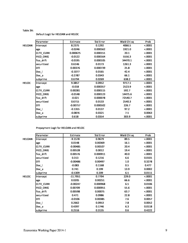
Regression Analysis–Default Probability Our general approach is to estimate a multinomial logit for our probability of default model and employ OLS to estimate LGD for those loans that have defaulted. As these methods are widely used in the literature, we do not present details here, but will include a more complete discussion of methodological choice in the next version of this paper. We estimated default and prepayment for HELOAN and HELOC separately, controlling for loan age, current combined LTV (CCLTV), original FICO, change in FICO since origination (FICO_DRIFT), DTI, whether underwriting included income and asset verification or not (DOC_I and DOC_A), whether the loan was subprime or not, and whether the loan is securitized or not. We treat HELOAN and HELOC as two distinct loan segments, since HELOAN behaves more like traditional mortgages, while HELOC has the initial draw period until the loan limit is reached and is then followed by an amortization period, so sensitivities and timing of default and prepayment may well be very different between these two product groups.
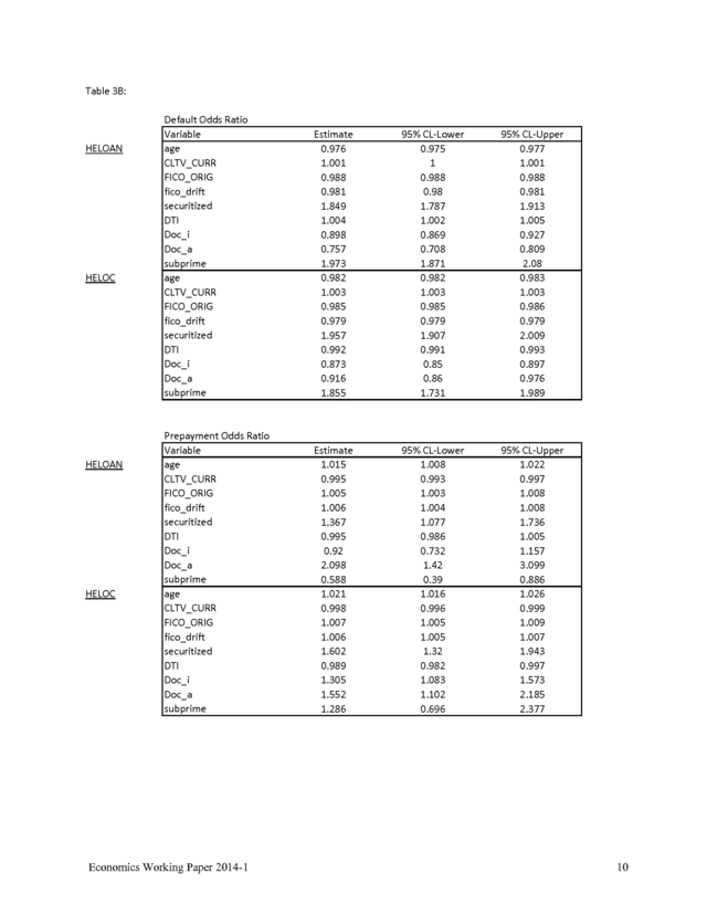
Results appear in tables 3A and 3B on the next page. Table 3A provides coefficients and standard errors. Table 3B provides odds ratios, the typical method for evaluating the effect of indicator variables on the loan status dependent variable when using a logit model.
We discuss results following the tables. Economics Working Paper 2014-1 8 . Table 3A: Default Logit for HELOAN and HELOC HELOAN HELOC Parameter Intercept age CLTV_CURR FICO_ORIG fico_drift securitized DTI Doc_i Doc_a subprime Intercept age CLTV_CURR FICO_ORIG fico_drift securitized DTI Doc_i Doc_a subprime Estimate 8.2375 -0.0246 0.000675 -0.0122 -0.0195 0.6146 0.00376 -0.1077 -0.2787 0.6794 9.3857 -0.018 0.00281 -0.0148 -0.021 0.6715 -0.00757 -0.1355 -0.0876 0.618 Std Error 0.1292 0.000562 0.000151 0.000164 0.000105 0.0173 0.000739 0.0165 0.0343 0.0269 0.0952 0.000357 0.000115 0.000123 0.000078 0.0133 0.000502 0.0137 0.0321 0.0354 Wald Chi-sq 4066.5 1921.0 20.1 5556.3 34470.1 1261.3 25.8 42.4 66.1 638.2 9717.1 2523.9 592.7 14475.6 72540.7 2540.3 226.7 97.2 7.5 303.9 Prob <.0001 <.0001 <.0001 <.0001 <.0001 <.0001 <.0001 <.0001 <.0001 <.0001 <.0001 <.0001 <.0001 <.0001 <.0001 <.0001 <.0001 <.0001 0.0063 <.0001 Std Error 0.9679 0.00369 0.00107 0.0012 0.000911 0.1216 0.00497 0.1168 0.199 0.209 0.7794 0.00251 0.000968 0.000951 0.00075 0.0986 0.00385 0.0953 0.1746 0.3135 Wald Chi-sq 89.5 16.1 20.4 19.4 40.0 6.6 1.0 0.5 13.9 6.5 229.0 66.6 6.5 55.6 63.7 22.8 7.6 7.8 6.3 0.6 Prob <.0001 <.0001 <.0001 <.0001 <.0001 0.0101 0.3278 0.477 0.0002 0.0111 <.0001 <.0001 0.0106 <.0001 <.0001 <.0001 0.0057 0.0052 0.0118 0.4222 Prepayment Logit for HELOAN and HELOC HELOAN HELOC Parameter Intercept age CLTV_CURR FICO_ORIG fico_drift securitized DTI Doc_i Doc_a subprime Intercept age CLTV_CURR FICO_ORIG fico_drift securitized DTI Doc_i Doc_a subprime Economics Working Paper 2014-1 Estimate -9.1578 0.0148 -0.00485 0.00528 0.00576 0.313 -0.00486 -0.083 0.741 -0.5309 -11.7951 0.0205 -0.00247 0.00709 0.00598 0.471 -0.0106 0.2662 0.4397 0.2516 9 . Table 3B: HELOAN HELOC HELOAN HELOC Default Odds Ratio Variable age CLTV_CURR FICO_ORIG fico_drift securitized DTI Doc_i Doc_a subprime age CLTV_CURR FICO_ORIG fico_drift securitized DTI Doc_i Doc_a subprime Estimate 0.976 1.001 0.988 0.981 1.849 1.004 0.898 0.757 1.973 0.982 1.003 0.985 0.979 1.957 0.992 0.873 0.916 1.855 95% CL-Lower 0.975 1 0.988 0.98 1.787 1.002 0.869 0.708 1.871 0.982 1.003 0.985 0.979 1.907 0.991 0.85 0.86 1.731 95% CL-Upper 0.977 1.001 0.988 0.981 1.913 1.005 0.927 0.809 2.08 0.983 1.003 0.986 0.979 2.009 0.993 0.897 0.976 1.989 Prepayment Odds Ratio Variable age CLTV_CURR FICO_ORIG fico_drift securitized DTI Doc_i Doc_a subprime age CLTV_CURR FICO_ORIG fico_drift securitized DTI Doc_i Doc_a subprime Estimate 1.015 0.995 1.005 1.006 1.367 0.995 0.92 2.098 0.588 1.021 0.998 1.007 1.006 1.602 0.989 1.305 1.552 1.286 95% CL-Lower 1.008 0.993 1.003 1.004 1.077 0.986 0.732 1.42 0.39 1.016 0.996 1.005 1.005 1.32 0.982 1.083 1.102 0.696 95% CL-Upper 1.022 0.997 1.008 1.008 1.736 1.005 1.157 3.099 0.886 1.026 0.999 1.009 1.007 1.943 0.997 1.573 2.185 2.377 Economics Working Paper 2014-1 10 . Probability of Default Preliminary Results–Discussion Signs and magnitudes of coefficients are generally consistent for both HELOAN and HELOC, and are generally as expected, although the age variable has a negative sign, probably reflecting the time period we study, during which house prices were declining so that newer originations experienced greater overall house price depreciation than older loans. The only variable that has different signs for HELOAN and HELOC is the DTI variable; it is positive for HELOAN, which behaves more like traditional mortgages, and negative for HELOC, possibly indicating that borrowers with greater need for liquidity are less likely to default on their lines of credit. As expected, borrower FICO score is negative and highly statistically significant in the default equation, but positive in the prepayment equation, confirming the often observed pattern that better borrowers are less likely to default but more likely to prepay, and vice-versa. Current LTV ratio is also highly statistically significant with expected signs. Borrowers with higher current LTVs are more likely to default but less likely to prepay. As mentioned earlier, we also have a measure of the borrower’s current credit score and calculate its change from the point of origination (FICO_DRIFT).
A decline in credit score may be viewed as a proxy for financial problems; an increase, for improvements in overall financial position. This proves to be a highly predictive variable, as it is certainly the most statistically significant variable in the default equations. Borrowers with declines in credit score are much more likely to default and borrowers with improved credit score are much more likely to prepay. Other variables not often available to researchers include method of loan underwriting; in particular, whether income and/or assets were documented (DOC_I; DOC_A). Consistent with an emerging literature (and common sense), verifying income and assets appears to reduce default risk, with odds ratios of between 0.70 and 0.92, respectively.
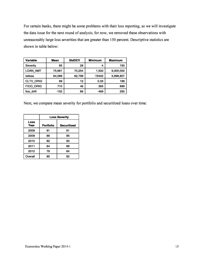
Results are less clear in the prepayment function, as both coefficients are positive, indicating greater prepayment risk, but the coefficients are not all significant at the 5 percent level. Economics Working Paper 2014-1 11 . As stated in the abstract, a key variable of interest is securitization. We find that securitized loans have both higher default and prepayment risk than portfolio loans, with odds ratios of 1.9-2.0 and 1.4-1.6, respectively, which is even higher than the odds ratio for the “subprime” variable. We will refine these estimates, adding control variables as necessary and tests for sample selection bias. 5. Loss Given Default Estimation Inspection of descriptive statistics suggests that LGD is higher for securitized loans.
In terms of a raw difference, we note a 92 percent mean loss severity for securitized loans, compared with an 85 percent loss severity rate for portfolio loans. Our effort here is to determine whether this difference persists after controlling for other factors that may affect loss severity. For the LGD regressions, we did not separately estimate equations for HELOAN and HELOC loans, since we believe that the behavioral patterns for LGD are sufficiently homogeneous between these two groups. Data Our dataset is necessarily smaller, since we only have realized losses for loans that defaulted. After excluding cases with important covariates missing, we have approximately 70,000 observations.
Lenders typically booked losses over several months following a 90-day delinquency status (sometimes later). To arrive at the total loss amount, we summed these writedowns over time. Due to some data problems with missing values for current loan balance, we define loss severity as the total loss amount as a fraction of initial loan amount.
In future revisions, and as our problem with missing current loan balances is resolved, we will employ the more traditional loss severity definition, namely the total loss amount as a fraction of balance at time of default. In order to avoid large influential observations that could alter our regression results, we performed data cleaning on the dataset to only use observations within the 1st percentile and 99th percentile. For example, loans with original balances of less than $1,000 are deleted, and severities less than -4 percent are eliminated.
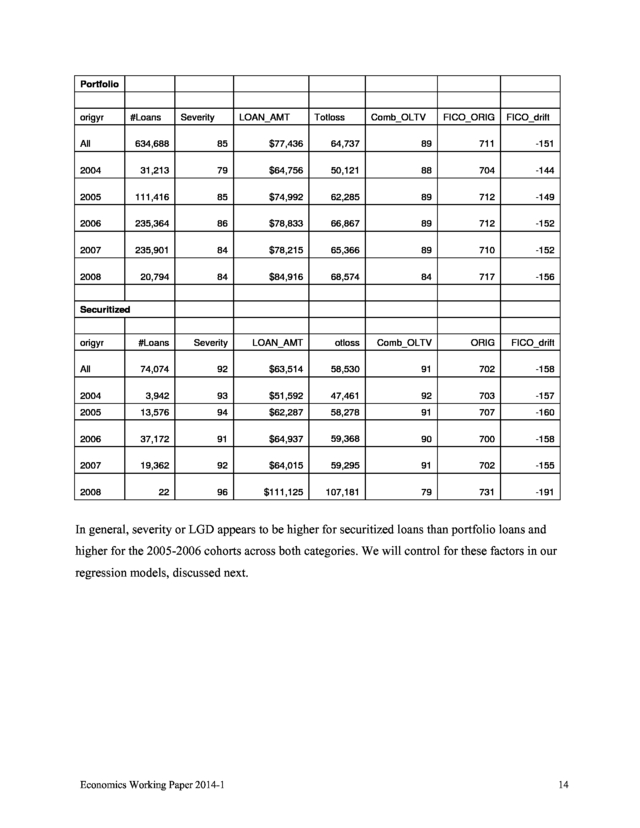
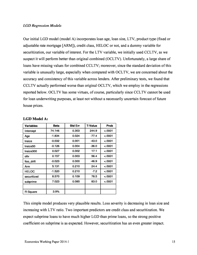
After these cleaning procedures, we still noticed that there are about 5 percent of loans with loss severity greater than 150 percent. Economics Working Paper 2014-1 12 . For certain banks, there might be some problems with their loss reporting, so we will investigate the data issue for the next round of analysis; for now, we removed these observations with unreasonably large loss severities that are greater than 150 percent. Descriptive statistics are shown in table below: Variable Mean Severity StdDEV Minimum Maximum 85 28 -4 150 LOAN_AMT 75,981 70,254 1,500 9,000,000 totloss 64,089 62,799 -15402 5,898,807 CLTV_ORIG 89 12 0.05 199 FICO_ORIG 710 46 365 899 -152 66 -469 250 fico_drift Next, we compare mean severity for portfolio and securitized loans over time: Loss Severity Loss Year Portfolio Securitized 2008 91 91 2009 89 95 2010 82 93 2011 84 88 2012 79 84 Overall 85 92 Economics Working Paper 2014-1 13 . Portfolio origyr All #Loans Severity LOAN_AMT Totloss Comb_OLTV FICO_ORIG FICO_drift 634,688 85 $77,436 64,737 89 711 -151 2004 31,213 79 $64,756 50,121 88 704 -144 2005 111,416 85 $74,992 62,285 89 712 -149 2006 235,364 86 $78,833 66,867 89 712 -152 2007 235,901 84 $78,215 65,366 89 710 -152 2008 20,794 84 $84,916 68,574 84 717 -156 origyr #Loans Severity LOAN_AMT otloss Comb_OLTV ORIG FICO_drift All 74,074 92 $63,514 58,530 91 702 -158 2004 3,942 93 $51,592 47,461 92 703 -157 2005 13,576 94 $62,287 58,278 91 707 -160 2006 37,172 91 $64,937 59,368 90 700 -158 2007 19,362 92 $64,015 59,295 91 702 -155 2008 22 96 $111,125 107,181 79 731 -191 Securitized In general, severity or LGD appears to be higher for securitized loans than portfolio loans and higher for the 2005-2006 cohorts across both categories. We will control for these factors in our regression models, discussed next. Economics Working Paper 2014-1 14 . LGD Regression Models Our initial LGD model (model A) incorporates loan age, loan size, LTV, product type (fixed or adjustable rate mortgage [ARM]), credit class, HELOC or not, and a dummy variable for securitization, our variable of interest. For the LTV variable, we initially used CCLTV, as we suspect it will perform better than original combined (OCLTV). Unfortunately, a large share of loans have missing values for combined CCLTV; moreover, since the standard deviation of this variable is unusually large, especially when compared with OCLTV, we are concerned about the accuracy and consistency of this variable across lenders. After preliminary tests, we found that CCLTV actually performed worse than original OCLTV, which we employ in the regressions reported below.
OCLTV has some virtues, of course, particularly since CCLTV cannot be used for loan underwriting purposes, at least not without a necessarily uncertain forecast of future house prices. LGD Model A: Beta Std Err T-Value Prob Intercept 74.146 0.303 244.9 <.0001 Age -1.834 0.024 -77.4 <.0001 lnsize -0.032 0.001 -43.0 <.0001 lnsize50 -0.126 0.004 -36.0 <.0001 lnsize300 0.027 0.002 17.1 <.0001 oltv 0.157 0.003 56.4 <.0001 -0.023 0.000 -46.9 <.0001 5.131 0.210 24.4 <.0001 -1.520 0.210 -7.2 <.0001 securitized 8.570 0.109 78.5 <.0001 subprime 7.023 0.085 83.0 <.0001 R-Square 3.9% Variables fico_drift Arm HELOC This simple model produces very plausible results. Loss severity is decreasing in loan size and increasing with LTV ratio. Two important predictors are credit class and securitization.
We expect subprime loans to have much higher LGD than prime loans, so the strong positive coefficient on subprime is as expected. However, securitization has an even greater impact. Economics Working Paper 2014-1 15 . Adjustable rate instruments (ARM) have higher LGD, whereas HELOCs generate lower LGD. This is consistent with the literature that HELOC loans are generally extended to higher income and higher credit score borrowers. Lastly, the change in the borrower’s financial condition since origination as captured by FICO_DRIFT is highly significant, as credit degradation increases LGD. Building on this baseline specification, we then added current note rate, a flag for loan modification, and other controls, including state dummy variables (not reported below, in the interest of table brevity) and loss-year dummies. Together, these latter two sets of dummy variables should capture cross-sectional variation in housing market conditions and the statelevel legal environment, as well as the overall time trend in housing market conditions. The current note rate proved to be a highly significant variable, since the higher the note rate, the higher the lost interest accrual, adding to losses.
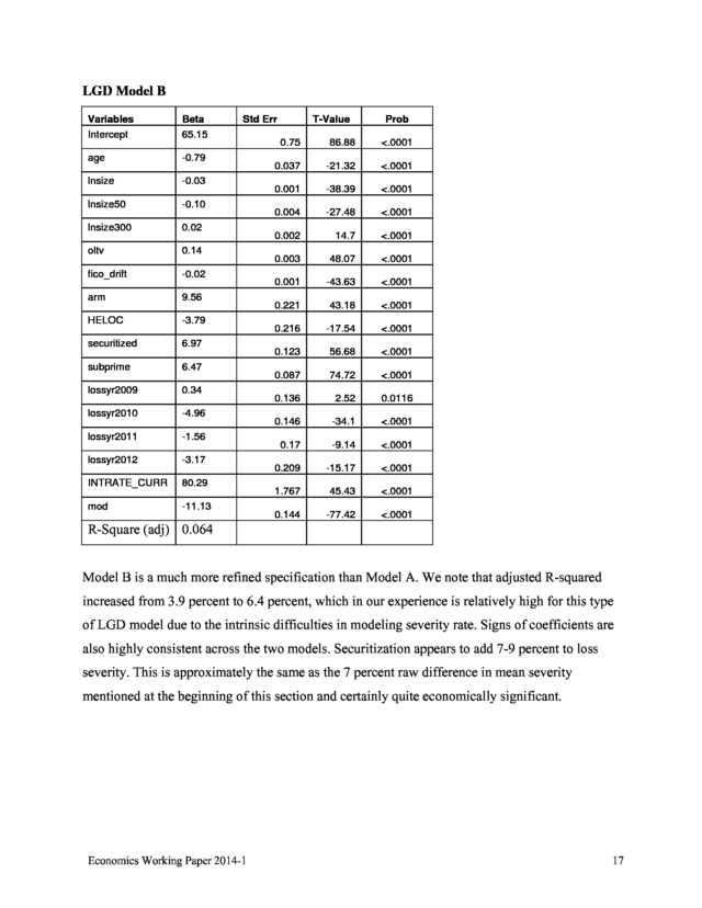
About 7 percent of loans are flagged as having been modified through rate reduction, term change, or principal reduction. A dummy variable for loan modification also proves highly significant, with an impact of -11 percent on the severity rate. While not reported, results of the state dummy variables are consistent with expectations. For example, the so-called “sand states” of Arizona, California, Florida, and Nevada all have large and statistically significant positive coefficients.
Likewise, states relatively less affected by the market downturn and with more rapid foreclosure procedures, for example, Texas, have a large and statistically significant negative coefficient. Economics Working Paper 2014-1 16 . LGD Model B Variables Intercept Beta 65.15 age -0.79 lnsize -0.03 lnsize50 -0.10 lnsize300 0.02 oltv 0.14 fico_drift -0.02 arm 9.56 HELOC -3.79 securitized 6.97 subprime 6.47 lossyr2009 0.34 lossyr2010 -4.96 lossyr2011 -1.56 lossyr2012 -3.17 INTRATE_CURR 80.29 mod Std Err -11.13 R-Square (adj) 0.064 T-Value Prob 0.75 86.88 <.0001 0.037 -21.32 <.0001 0.001 -38.39 <.0001 0.004 -27.48 <.0001 0.002 14.7 <.0001 0.003 48.07 <.0001 0.001 -43.63 <.0001 0.221 43.18 <.0001 0.216 -17.54 <.0001 0.123 56.68 <.0001 0.087 74.72 <.0001 0.136 2.52 0.0116 0.146 -34.1 <.0001 0.17 -9.14 <.0001 0.209 -15.17 <.0001 1.767 45.43 <.0001 0.144 -77.42 <.0001 Model B is a much more refined specification than Model A. We note that adjusted R-squared increased from 3.9 percent to 6.4 percent, which in our experience is relatively high for this type of LGD model due to the intrinsic difficulties in modeling severity rate. Signs of coefficients are also highly consistent across the two models. Securitization appears to add 7-9 percent to loss severity.
This is approximately the same as the 7 percent raw difference in mean severity mentioned at the beginning of this section and certainly quite economically significant. Economics Working Paper 2014-1 17 . 6. Conclusion and Extensions In this paper, we have sampled from a very large database of home equity mortgage loans made by the largest commercial banks in the U.S. We examined loan performance, including LGD for home equity loans, whether securitized or held in portfolio by the originator. We find an increase in the probability of default among those loans that were securitized, and higher loss severity among such loans as well. We have additional work to do.
While initial results for the probability of default model are encouraging, we need to incorporate interaction variables and otherwise test the specification to ensure robustness of results. More importantly, we have not yet addressed potential sample selectivity issues. If securitized home equity loans are systematically different than loans held in portfolio, our initial modeling approach may be inappropriate.
Hence, we need to model the lender’s securitization decision. We plan to rely on the established literature (Ambrose, LaCourLittle, and Sanders [2005] and Agrawal, Chang, and Yavas [2012]) to do so. Essentially, this method is to develop models that lenders could have used at time of origination (hence, without updated collateral values or changes to credit scores) to estimate default and prepayment, and compare predicted probabilities with loan pricing; i.e., to assume lenders rationally retain loans that have better risk and return profiles.
A final issue of possible sample selectivity relates to the OCC Mortgage Metrics database itself. Since that database begins tracking loans only in 2008, it is subject to potential survivorship bias if loans that terminated prior to 2008 are systematically different from those whose performance we examine. Survivorship issues are a common problem in the mortgage loan performance literature and we anticipate using standard methods to test and/or correct our results. Economics Working Paper 2014-1 18 .
References Agarwal, Sumit, Yan Chang, and Abdullah Yavas. 2012. “Adverse Selection in Mortgage Securitization.” Journal of Financial Economics 105(3): 640-660. Agarwal, Sumit, Brent Ambrose, S. Chomsisengphet, and C.
Liu. 2006. “An Empirical Analysis of Home Equity Loan and Line Performance.” Journal of Financial Intermediation 15: 444-469. Agarwal, Sumit, Brent Ambrose, S.
Chomsisengphet, and C. Liu. 2005.
“Credit Lines and Credit Utilization.” Journal of Money, Credit and Banking 38(1): 1-22. Agarwal, Sumit, Brent Ambrose, Chomsisengphet, S., and Liu, C. 2011. “The Role of Soft Information in a Dynamic Contract Setting: Evidence from the Home Equity Credit Market.” Journal of Money, Credit and Banking 43(4): 633-655. Altman, Edward I.
2001.“Altman High Yield Bond and Default Study,” Salomon Smith Barney, U.S. Fixed Income High Yield Report, July. Altman, E. and G.
Fanjul. 2004. “Defaults and Returns in the High Yield Bond Market: Analysis Through 2003,” NYU Salomon Center Working Paper, January (also through 2003 Q3). Altman, Edward, Andrea Resti, and Andrea Sironi.
2003. “Default Recovery Rates In Credit Risk Modeling: A Review of the Literature and Empirical Evidence,” Working Paper, New York University. Ambrose, Brent W., and Michael LaCour-Little. 2005.
“A Note on Hybrid Mortgages.” Real Estate Economics 33(4): 265-290. Ambrose, Brent W., Michael LaCour-Little, and Anthony Sanders. 2005. “The Effect of Conforming Loan Status on Mortgage Yield Spreads: A Loan Level Analysis,” Real Estate Economics 32: 541-569. Bellotti, Tony and Jonathan Crook.
2009. “Loss Given Default Models for UK Retail Credit Cards,” Working Paper, Credit Research Centre, University of Edinburgh Business School. Calem, Paul S. and Michael LaCour-Little.
2004. “Risk Based Capital Requirements for Mortgage Loans.” Journal of Banking & Finance 28: 647-672. Canner, G.B., J.T. Fergus, and C.A.
Luckett. 1988. “Home Equity Lines of Credit.” Federal Reserve Bulletin, June, 361-373. Carey, Mark and Michael Gordy.
2003. “Systematic Risk in Recoveries on Defaulted Debt,” mimeo, Federal Reserve Board, Washington. Economics Working Paper 2014-1 19 . Cooper, D. 2010. “Did Easy Credit Lead to Overspending? Home Equity Borrowing and Household Behavior in the Early 2000s,” Federal Reserve Bank of Boston, Working Paper No. 09-7. Crawford, Fordon W. and Eric Rosenblatt.
1995. “Efficient Mortgage Default Option Exercise: Evidence from Loss Severity.” The Journal of Real Estate Research 10(5): 543-555. Fitch Ratings, 2012. U.S.
Housing and Bank Balance Sheets Special Report, February 27, 2012. Frye, John (2000a), “Collateral Damage,” Risk, April, 91-94. Frye, John (2000b), “Collateral Damage Detected,” Federal Reserve Bank of Chicago, Working Paper, Emerging Issues Series, October, 1-14. Goodman, L., R. Ashworth, B. Landy, and K.
Yin. 2010. “Second Liens: How Important?” The Journal of Fixed Income 20 (2), Fall: 19-30. Gordy, Michael B.
and Bradley Howells. 2004. “Procyclicality in Basel II: Can We Treat the Disease Without Killing the Patient?” Greenspan, A.
and J. Kennedy. 2008.
“Sources and Uses of Equity Extracted from Homes.” Oxford Review of Economic Policy 24 (1): 120-144. Inside Mortgage Finance, 2013. Chart of the Week: Non-Agency MBS Characteristics. March 26, 2013. Keys, Benjamin, Tanmoy Mukherjee, Amit Seru, and Vikrant Vig.
2010. “Did Securitization Lead to Lax Screening?” The Quarterly Journal of Economics 125 (1): 307-362. Keys, Benjamin, Amit Seru, and Vikrant Vig. 2012.
“Lender Screening and the Role of Securitization: Evidence from Prime and Subprime Mortgage Markets.” Review of Financial Studies (2012) 25(7): 2071-2108. Ji, Lu and Yanan Zhang. 2010. “Basel II Loss Given Default Modeling of Seasoned Residential Mortgage Loans,” Working Paper. LaCour-Little, M., 2004.
“Equity Dilution: An Alternative Perspective on Mortgage Default.” Real Estate Economics 32(3): 359-384. LaCour-Little, Michael, Eric Rosenblatt, and Vincent Yao. 2010. “Equity Extraction by Homeowners: 2000-2006.” Journal of Real Estate Research 32(1): 23-46. LaCour-Little, Michael, Libo Sun, and Wei Yu.
2013. “The Role of Home Equity Lending in the Recent Mortgage Crisis.” Real Estate Economics, forthcoming. Economics Working Paper 2014-1 20 . LaCour-Little, Michael, Charles A. Calhoun, and Wei Yu. 2011. “What Role Did Piggyback Lending Play in the Housing Bubble and Mortgage Collapse?” Journal of Housing Economics 20(2): 81-100. Lekkas, Vassilis, John M.
Quigley, and Robert Van Order. 1993 “Loan Loss Severity and Optimal Mortgage Default.” Journal of the American Real Estate Research and Urban Economics Association 21(4): 353-371. Mian, A.R., A. Sufi.
2009. “The Consequences of Mortgage Credit Expansion: Evidence from the U.S. Mortgage Default Crisis.” Quarterly Journal of Economics, 124(4): 1449-1496. Mian, A.R., A.
Sufi. 2011. “House Prices, Home Equity-Based Borrowing, and the U.S. Household Leverage Crisis.” American Economic Review, 101: 2132-2156. Pennington-Cross, Anthony.
2003. “Subprime and Prime Mortgages: Loss Distributions,” unpublished manuscript, May. Pennington-Cross, Anthony. 2006.
“The Duration of Foreclosure in the Subprime Mortgage Market: A Competing Risks Model with Mixing,” Working Paper, Federal Reserve Bank of St. Louis. Qi, Min and Xiaolong Yang. 2009. “Loss Given Default of High Loan-to-Value Residential Mortgages.” Journal of Banking and Finance 33(5): 788–799. Saurina, Jesus and Gabriel Jimenez.
2006. “Credit Cycles, Credit Risk, and Prudential Regulation.” International Journal of Central Banking, June 2006. Schuermann, Til. 2004.
“What Do We Know About Loss Given Default?” Working Paper, Wharton Financial Institutions Center. Weicher, John C. 1997. The Home Equity Lending Industry.
The Hudson Institute: Indianapolis, Indiana. Economics Working Paper 2014-1 21 .
The authors take responsibility for any errors. . Default Probability and Loss Given Default for Home Equity Loans Michael LaCour-Little Yanan Zhang June 2014 Abstract: Securitization has been widely assigned blame for contributing to the recent mortgage market meltdown and ensuing financial crisis. In this paper, we sample from the OCC Mortgage Metrics database to develop estimates of default probabilities and loss given default for home equity loans originated during 2004-2008 and tracked from 2008-2012. We are particularly interested in the relationship between loan outcomes and the lender’s decision to securitize the asset. Among other innovations, we are able to measure the change in the borrower’s credit score over time and the level of documentation used during loan underwriting.
Results suggest that securitized home equity loans bear higher default risk and produce greater loss severity than loans held in portfolio by lenders. Economics Working Paper 2014-1 i . 1. Introduction Securitization, particularly non-agency securitization of subprime and Alt-A mortgages, has been identified as a contributory factor in the recent financial crisis (see, for example, Keys, Mukherjee, Seru, and Vig [2010] or Keys, Seru, and Vig [2012]). While first mortgage loans have been widely studied, home equity loans have not. The current paper addresses this gap in the literature utilizing the Office of the Comptroller of the Currency (OCC) Mortgage Metrics dataset.
To preview our main result, we find that securitized home equity loans do have greater default probability (PD) and loss given default (LGD) than loans retained in portfolio by major banks. While less frequently studied than first mortgages, home equity loans grew rapidly during the period 2000-2008 and became a sizable segment of the mortgage market. The total dollars outstanding of home equity loans increased from $275.5 billion in 2000 to a peak of $953.5 billion in 2008, an average annual growth rate of 16.8 percent. Likewise, the total number of home equity loans increased from 12.9 million in 2000 to a peak of 23.8 million in 2007, an average annual growth rate of 9.1 percent.
Since balances were growing faster than accounts, average loan size was increasing over the period as well. Unlike first lien loans, the majority of which are securitized, most home equity loans remain on bank balance sheets. Aggregate bank risk exposure to home equity loans is estimated to be 30 percent of the total residential mortgage exposure, or roughly $750 billion (Fitch Ratings, 2012).
As the private-label mortgage securitization market has recently shown signs of resurgence, home equity loans are again evident (Inside Mortgage Finance, 2013). Research has also shown that junior lien lending through home equity loans is related to the documented increase in household leverage (Mian and Sufi [2011]) and to the much-reported decline in personal savings (Greenspan and Kennedy [2008]). Moreover, increased debt usage through home equity lending can also dilute equity in a borrower’s home, thereby increasing the default risk of first mortgages and magnifying the impact of declining house prices on default and foreclosure rates (LaCour-Little [2004]). Likewise, LaCour-Little, Sun, and Yu (2013) find Economics Working Paper 2014-1 1 .
that greater home equity lending at the zip code level, especially of home equity lines of credit (HELOC), is related to higher rates of mortgage default on first mortgages in the same area. Our contribution in this paper is to examine the PD and loss severity of home equity loans during the recent market downturn, 2008-2012. Among other enhancements, we have a measure of borrower credit score over time, allowing us a rough proxy for changes in the borrower’s financial position prior to default. Moreover, we have measures of income and asset verification, so that we can quantify the role of reduced documentation in default risk. The paper is organized as follows. In the next section, we review the literature on mortgage loan performance, and the more limited research on LGD generally and home equity lending in particular.
In the third section, we describe our data and sampling approach. In Section IV, we present regression models of PD and discuss results. Section V presents the data used and regression models estimated for LGD estimates, including a discussion of results.
Section VI presents conclusions and extensions in progress. 2. Literature Review PD and LGD on fixed income instruments are a longstanding topic of interest in finance. For example, Altman, Resti, and Sironi (2003) present a broad review of the literature and the empirical evidence of default recovery rates in credit-risk modeling.
Their paper focuses on the relationship between PD and LGD and how this relationship is treated in different modeling frameworks. Recent empirical evidence cited suggests that LGD is positively correlated with PD. 1 The evolving Basel standards have stimulated additional research on LGD.
Schuermann (2004), for example, analyzes the definition and measurement of LGD in the context of Basel II and analyzes data from Moody’s Default Risk Service Database. Among his findings, he reports that 1 See details of the empirical evidence in Frye (2000a, b), Jarrow (2001), Carey and Gordy (2003), and Altman et al. (2001, 2004). Economics Working Paper 2014-1 2 . the recovery distribution is bimodal, lower in recessions than in expansions. Both the Altman and Schuermann papers are based on corporate bond data. Relatively fewer papers focus on consumer loans, such as credit card or home mortgage debt, although this literature is growing rapidly. This is probably due to the absence of publicly available data, since most of these loans reside on bank balance sheets, and lender focus on PD modeling. An early paper that is focused on LGD for residential mortgages is Lekkas et al. (1993).
They test the frictionless options-based mortgage default theory empirically and report that higher loss severity is associated with higher original loan-to-value (LTV), geographical locations with higher default rates, and younger mortgage loans. Crawford and Rosenblatt (1995) incorporate transaction costs into the options-based mortgage default model and empirically test its effect on loss severity. Among their findings is that LGD is reduced where the probability of a deficiency judgment is higher.
Among more recent papers focused on mortgage loans, Calem and LaCour-Little (2004) also analyze the determinants of LGD. Their regression results confirm Lekkas et al. (1993) for either original LTV or combined loan-to-value (CLTV).
They also report that both mortgage age and loan size have significant effects on LGD, with smaller loans exhibiting higher loss severity due to fixed costs associated with exercising the foreclosure option. More recently, Qi and Yang (2009) study LGD of high LTV loans using data from private mortgage insurance companies. They find that CLTV is the single most important determinant of LGD. They find that mortgage loss severity in distressed housing markets is significantly higher than under normal housing market conditions.
In a study unrelated to mortgage lending, Bellotti and Crook (2009) study LGD models for UK retail credit cards. They compare several econometric methods for modeling LGD and find that Ordinary Least Squares models with macroeconomic variables perform best to forecast LGD at both the account level and the portfolio level. The inclusion of macroeconomic variables enables them to model LGD in downturn conditions as required by Basel II. Most of these studies have focused on testing particular theories and underlying relationships. Studies on business cycle effects remain limited, although there have been some attempts to test Economics Working Paper 2014-1 3 .
the downturn effect. For example, Calem and LaCour-Little (2004) examine the relationship between LGD and the economic environment using simulation at the portfolio level. Qi and Yang (2009), cited above, test the effect of housing market downturns by inclusion of a dummy variable. For home equity lending specifically, the literature is much more limited. Canner, Fergus, and Luckett (1988) describe the early stages and growth of the home equity lending segment, following passage of the 1986 tax law changes which are generally acknowledged to have accelerated the growth of this segment of consumer lending.
2 Weicher (1997) reviews the home equity lending industry during the 1990s, characterizing it as business based on recapitalizing borrowers with impaired credit but substantial housing equity. LaCour-Little, Calhoun, and Yu (2011) focus on simultaneous close or “piggyback” loans, and find that such lending is associated with higher default and foreclosure rates in subsequent years. Goodman, Ashworth, Landy, and Yin (2010) report that the presence of junior lien mortgages increases the default risk of first lien mortgages.
Ambrose, Agrawal, and Liu (2005) show that patterns of home equity line use are also related to borrower credit quality, as measured by their FICO scores. Extending that analysis further, Agarwal, Ambrose, Chomsisengphet, and Liu (2006) examine the performance of home equity lines and loans, finding considerable difference in terms of default and prepayment risk. Agarwal, Ambrose, Chomsisengphet, and Liu (2010) examine the role of soft information in home equity lending and find that its use can be effective in reducing default risk.
LaCour-Little, Rosenblatt, and Yao (2010) document the magnitude of equity extraction by homeowners during the period 2000-2006. Cooper (2010) finds that high equity extraction has been used both for household expenditures and home improvement during the 2000-2006 housing boom. The present paper contributes to the existing literature on LGD and home equity lending in the following ways. First, we sample from a comprehensive dataset of mortgage lending by the largest commercial banks in the U.S.
Second, due to the richness of this dataset, we are able to employ a reasonable proxy for the financial positions of households utilizing their current credit 2 Prior to 1986, most interest on consumer debt was tax-deductible; after the 1986 tax law changes, only residential mortgage debt remained generally deductible for those who itemize deductions. Economics Working Paper 2014-1 4 . scores. Third, we have measures for the level of documentation used in loan underwriting, allowing us to quantify the effect of “low doc” underwriting on default risk. Finally, since we have information on whether the loan was securitized or not, we are able to examine the correlates of that decision on subsequent loan performance. 3. Data and Sampling Scheme The data used in this research is a sample taken from the OCC’s Mortgage Metrics database. This is a loan-level dataset of monthly servicing information from nine large national banks assembled by LPS Applied Analytics and provided to the OCC.
The database is quite rich and contains more than 80 fields. Variables denote the borrower’s credit profile, loan product details, collateral information, and loan performance history, including both delinquency and loan modification information. Collection of monthly performance information began in May 2008 and continues to the present; accordingly, we will be able to update results as more time passes. The underlying loans account for two-thirds of the overall home equity market, and there are more than 9 million loan records added to the database each month.
This is truly “big data.” In table 1A, we present a snapshot of the database as of December 2009 to better illustrate the distribution of loans in the database. There are 10.5 million loans in active status at the end of 2009; of these, 8.2 million are in second lien position; of these, 7.2 million were originated between 2004 and 2008 and are either held in portfolio or securitized by private issuers. Of the 7.2 million second liens, 2.0 million, or about 28 percent, are home equity loans (sometimes called closed end seconds or CES), and the rest are HELOCs. Economics Working Paper 2014-1 5 .
LOAN_OWNER All LoanCount Avg Balance INTRATE_ INTRATE_C CLTV_ CLTV_C FICO_O FICO_C ORIG URR ORIG URR RIG URR DTI arm Income Asset Document Document ed ed subprime All 7,215,037 $56,001 7.29% 5.14% 78.6 74.7 735 717 36.6 73.5% 6.6% 25.3% 11.8% Securitized 542,302 $46,579 7.20% 7.54% 86.2 97.9 715 685 35.7 66.6% 3.0% 39.0% 3.5% Portfolio 6,672,735 $56,762 7.30% 4.94% 78.0 72.8 736 720 36.6 74.1% 6.9% 24.2% 12.5% HE Loan All 2,005,284 $48,522 8.17% 8.00% 84.3 86.9 724 702 36.6 5.7% 14.6% 40.7% 17.3% %Sec'tzd Securitized 182,282 $43,077 8.42% 8.60% 89.2 88.3 713 678 37.3 0.5% 7.8% 48.8% 7.8% Portfolio 1,823,002 $49,057 8.15% 7.94% 83.9 86.7 725 704 36.5 6.2% 15.2% 39.9% 18.3% %Sec'tzd 7.5% 9.1% HELOC %Sec'tzd 6.9% All 5,209,753 $58,870 6.91% 4.03% 76.5 70.6 739 723 36.5 99.7% 3.6% 19.4% 9.7% Securitized 360,020 $48,319 6.62% 7.01% 84.8 102.4 716 689 35.0 100.0% 0.6% 34.0% 1.3% Portfolio 4,849,733 $59,653 6.93% 3.81% 75.8 68.1 741 726 36.7 3.8% 18.3% 10.3% 99.6% The share of securitized loans overall is 7.5 percent. The next table shows how securitization patterns and average loan characteristics have evolved over time. LoanCount AvgBal INTRATE_ INTRATE_ CLTV_ CLTV_C FICO_ FICO_C CURR ORIG ORIG URR ORIG URR origyr securitized DTI arm subprime Doc_i Doc_a 2003 No 533,121 $39,113 5.10% 4.29% 75 51 739 744 32 83% 4% 20% 14% 2003 Yes 42,896 $24,719 4.35% 5.34% 82 72 725 716 32 89% 1% 45% 1% 2004 No 812,061 $47,084 5.40% 4.26% 77 60 737 733 35 86% 6% 22% 15% 2004 Yes 71,001 $35,997 4.83% 6.02% 85 93 719 698 35 94% 5% 46% 9% 2005 No 1,323,251 $55,931 6.87% 4.64% 79 72 735 723 36 78% 9% 24% 14% 2005 Yes 107,594 $45,482 6.38% 7.54% 86 106 715 680 35 91% 8% 43% 8% 2006 No 1,628,302 $61,651 8.20% 5.27% 79 77 733 709 38 68% 10% 21% 11% 2006 Yes 208,498 $52,215 8.27% 8.17% 87 96 711 676 37 52% 2% 35% 2% 2007 No 1,793,137 $61,202 8.38% 5.53% 80 82 733 707 38 65% 6% 24% 10% 2007 Yes 112,300 $52,299 8.48% 8.20% 88 107 716 689 36 44% 0% 35% 0% 2008 No 582,863 $60,971 6.12% 4.43% 72 70 753 742 36 84% 2% 42% 16% 2008 Yes 13 $448,810 3.17% 6.80% 21 49 733 642 42 31% 46% 100% 100% Sampling from the Database In this section we briefly describe the construction of the dataset we use for this research. We include data cleaning and the creation of the panel dataset itself. Data Cleaning Whenever large datasets are involved, data cleaning is necessary. Upon sanity checking of the dataset, we noticed data anomalies and outliers that are better left out of the regression analysis. Since we are dealing with a large dataset, it is safe to leave out observations that are below 1 Economics Working Paper 2014-1 6 .
percentile or beyond 99 percentile. For HELOAN and HELOC portfolios respectively, these are the p1 and p99 values for key numeric variables used in the regression analysis. HELOAN cltv_curr cltv_orig DTI intrate_curr intrate_orig loanamt p1 2 15 7 0.041 0.056 7 p99 195 100 60 0.126 0.126 60 HELOC cltv_curr cltv_orig DTI intrate_curr intrate_orig loanamt p1 2 30 7 0.023 0.036 7 p99 195 100 70 0.13 0.13 70 Our data cleaning rules are largely based on the above table, and in some instances we relaxed the p1 or p99 constraint and selected a value smaller than the p1 value or greater than the p99 value if these values did not seem to be extreme values. For example, instead of using the p1 value of 0.041 for the lower bound of current interest rate, we only require this lower bound to be greater than zero, since lower interest rates may well be teaser rates and are not data anomalies. We have learned that teaser rates are small but never are zero, so we require a valid interest rate to be greater than zero. The upper bound for interest rates we chose is 0.13, consistent with the p99 value.
For current LTV, we require it to be between 2 and 195, as the p1 and p99 values suggest. For original LTV, we selected values between 1 and 100, where 100 is the p99 value, while 1 is closer to the minimum value. For debt-to-income ratio (DTI), we chose values between 7 and 100, as 7 is the p1 value and 100 is closer to the maximum value.
For loan amounts, we chose values that are larger than 7,000, the p1 value, while selecting everything up to the maximum value, which we assess to be reasonable. Creating the Balanced Panel for Modeling Panel data for securitized loans consist of 11.1 million loan months derived from 0.51 million unique loans. Since portfolio loans are more than 10 times the number securitized, we selected a random sample of portfolio loans of 0.51 million—the exact same number of loans as the securitized loans. The panel data of these portfolio loans consist of 10.7 million loan months.
We then pooled the securitized and held-in-portfolio loan months together, resulting in panel data of 22 million loan months. Of these, defaults occur in 207,000 loan months. In other words, we observe a loan default in slightly less than 1 percent of all loan months in the panel data sample, Economics Working Paper 2014-1 7 .
as defaults are over-weighted. In terms of gross lifetime default rate, this is about a 3 percent default rate based on the 7.2 million total loan count shown in table 1A. We kept all these loan months in our final estimation dataset and randomly selected the same number of loan months from the non-defaulted loan months. The result of this procedure is a final sample consisting of 414,000 loan months. At each point in time, we characterize loans in terms of their status, which initially takes on one of three values: currently active, defaulted, or paid off.
Default and paid off are the terminal states that we will model. There are additional subtleties to be considered; e.g., properties sold by their owners as short sales generally impose losses on lenders, yet those loans may not have actually defaulted prior to the short sale. Are such events defaults or prepayments? We will have to sort out such issues prior to the next version of this paper. 4.
Regression Analysis–Default Probability Our general approach is to estimate a multinomial logit for our probability of default model and employ OLS to estimate LGD for those loans that have defaulted. As these methods are widely used in the literature, we do not present details here, but will include a more complete discussion of methodological choice in the next version of this paper. We estimated default and prepayment for HELOAN and HELOC separately, controlling for loan age, current combined LTV (CCLTV), original FICO, change in FICO since origination (FICO_DRIFT), DTI, whether underwriting included income and asset verification or not (DOC_I and DOC_A), whether the loan was subprime or not, and whether the loan is securitized or not. We treat HELOAN and HELOC as two distinct loan segments, since HELOAN behaves more like traditional mortgages, while HELOC has the initial draw period until the loan limit is reached and is then followed by an amortization period, so sensitivities and timing of default and prepayment may well be very different between these two product groups.
Results appear in tables 3A and 3B on the next page. Table 3A provides coefficients and standard errors. Table 3B provides odds ratios, the typical method for evaluating the effect of indicator variables on the loan status dependent variable when using a logit model.
We discuss results following the tables. Economics Working Paper 2014-1 8 . Table 3A: Default Logit for HELOAN and HELOC HELOAN HELOC Parameter Intercept age CLTV_CURR FICO_ORIG fico_drift securitized DTI Doc_i Doc_a subprime Intercept age CLTV_CURR FICO_ORIG fico_drift securitized DTI Doc_i Doc_a subprime Estimate 8.2375 -0.0246 0.000675 -0.0122 -0.0195 0.6146 0.00376 -0.1077 -0.2787 0.6794 9.3857 -0.018 0.00281 -0.0148 -0.021 0.6715 -0.00757 -0.1355 -0.0876 0.618 Std Error 0.1292 0.000562 0.000151 0.000164 0.000105 0.0173 0.000739 0.0165 0.0343 0.0269 0.0952 0.000357 0.000115 0.000123 0.000078 0.0133 0.000502 0.0137 0.0321 0.0354 Wald Chi-sq 4066.5 1921.0 20.1 5556.3 34470.1 1261.3 25.8 42.4 66.1 638.2 9717.1 2523.9 592.7 14475.6 72540.7 2540.3 226.7 97.2 7.5 303.9 Prob <.0001 <.0001 <.0001 <.0001 <.0001 <.0001 <.0001 <.0001 <.0001 <.0001 <.0001 <.0001 <.0001 <.0001 <.0001 <.0001 <.0001 <.0001 0.0063 <.0001 Std Error 0.9679 0.00369 0.00107 0.0012 0.000911 0.1216 0.00497 0.1168 0.199 0.209 0.7794 0.00251 0.000968 0.000951 0.00075 0.0986 0.00385 0.0953 0.1746 0.3135 Wald Chi-sq 89.5 16.1 20.4 19.4 40.0 6.6 1.0 0.5 13.9 6.5 229.0 66.6 6.5 55.6 63.7 22.8 7.6 7.8 6.3 0.6 Prob <.0001 <.0001 <.0001 <.0001 <.0001 0.0101 0.3278 0.477 0.0002 0.0111 <.0001 <.0001 0.0106 <.0001 <.0001 <.0001 0.0057 0.0052 0.0118 0.4222 Prepayment Logit for HELOAN and HELOC HELOAN HELOC Parameter Intercept age CLTV_CURR FICO_ORIG fico_drift securitized DTI Doc_i Doc_a subprime Intercept age CLTV_CURR FICO_ORIG fico_drift securitized DTI Doc_i Doc_a subprime Economics Working Paper 2014-1 Estimate -9.1578 0.0148 -0.00485 0.00528 0.00576 0.313 -0.00486 -0.083 0.741 -0.5309 -11.7951 0.0205 -0.00247 0.00709 0.00598 0.471 -0.0106 0.2662 0.4397 0.2516 9 . Table 3B: HELOAN HELOC HELOAN HELOC Default Odds Ratio Variable age CLTV_CURR FICO_ORIG fico_drift securitized DTI Doc_i Doc_a subprime age CLTV_CURR FICO_ORIG fico_drift securitized DTI Doc_i Doc_a subprime Estimate 0.976 1.001 0.988 0.981 1.849 1.004 0.898 0.757 1.973 0.982 1.003 0.985 0.979 1.957 0.992 0.873 0.916 1.855 95% CL-Lower 0.975 1 0.988 0.98 1.787 1.002 0.869 0.708 1.871 0.982 1.003 0.985 0.979 1.907 0.991 0.85 0.86 1.731 95% CL-Upper 0.977 1.001 0.988 0.981 1.913 1.005 0.927 0.809 2.08 0.983 1.003 0.986 0.979 2.009 0.993 0.897 0.976 1.989 Prepayment Odds Ratio Variable age CLTV_CURR FICO_ORIG fico_drift securitized DTI Doc_i Doc_a subprime age CLTV_CURR FICO_ORIG fico_drift securitized DTI Doc_i Doc_a subprime Estimate 1.015 0.995 1.005 1.006 1.367 0.995 0.92 2.098 0.588 1.021 0.998 1.007 1.006 1.602 0.989 1.305 1.552 1.286 95% CL-Lower 1.008 0.993 1.003 1.004 1.077 0.986 0.732 1.42 0.39 1.016 0.996 1.005 1.005 1.32 0.982 1.083 1.102 0.696 95% CL-Upper 1.022 0.997 1.008 1.008 1.736 1.005 1.157 3.099 0.886 1.026 0.999 1.009 1.007 1.943 0.997 1.573 2.185 2.377 Economics Working Paper 2014-1 10 . Probability of Default Preliminary Results–Discussion Signs and magnitudes of coefficients are generally consistent for both HELOAN and HELOC, and are generally as expected, although the age variable has a negative sign, probably reflecting the time period we study, during which house prices were declining so that newer originations experienced greater overall house price depreciation than older loans. The only variable that has different signs for HELOAN and HELOC is the DTI variable; it is positive for HELOAN, which behaves more like traditional mortgages, and negative for HELOC, possibly indicating that borrowers with greater need for liquidity are less likely to default on their lines of credit. As expected, borrower FICO score is negative and highly statistically significant in the default equation, but positive in the prepayment equation, confirming the often observed pattern that better borrowers are less likely to default but more likely to prepay, and vice-versa. Current LTV ratio is also highly statistically significant with expected signs. Borrowers with higher current LTVs are more likely to default but less likely to prepay. As mentioned earlier, we also have a measure of the borrower’s current credit score and calculate its change from the point of origination (FICO_DRIFT).
A decline in credit score may be viewed as a proxy for financial problems; an increase, for improvements in overall financial position. This proves to be a highly predictive variable, as it is certainly the most statistically significant variable in the default equations. Borrowers with declines in credit score are much more likely to default and borrowers with improved credit score are much more likely to prepay. Other variables not often available to researchers include method of loan underwriting; in particular, whether income and/or assets were documented (DOC_I; DOC_A). Consistent with an emerging literature (and common sense), verifying income and assets appears to reduce default risk, with odds ratios of between 0.70 and 0.92, respectively.
Results are less clear in the prepayment function, as both coefficients are positive, indicating greater prepayment risk, but the coefficients are not all significant at the 5 percent level. Economics Working Paper 2014-1 11 . As stated in the abstract, a key variable of interest is securitization. We find that securitized loans have both higher default and prepayment risk than portfolio loans, with odds ratios of 1.9-2.0 and 1.4-1.6, respectively, which is even higher than the odds ratio for the “subprime” variable. We will refine these estimates, adding control variables as necessary and tests for sample selection bias. 5. Loss Given Default Estimation Inspection of descriptive statistics suggests that LGD is higher for securitized loans.
In terms of a raw difference, we note a 92 percent mean loss severity for securitized loans, compared with an 85 percent loss severity rate for portfolio loans. Our effort here is to determine whether this difference persists after controlling for other factors that may affect loss severity. For the LGD regressions, we did not separately estimate equations for HELOAN and HELOC loans, since we believe that the behavioral patterns for LGD are sufficiently homogeneous between these two groups. Data Our dataset is necessarily smaller, since we only have realized losses for loans that defaulted. After excluding cases with important covariates missing, we have approximately 70,000 observations.
Lenders typically booked losses over several months following a 90-day delinquency status (sometimes later). To arrive at the total loss amount, we summed these writedowns over time. Due to some data problems with missing values for current loan balance, we define loss severity as the total loss amount as a fraction of initial loan amount.
In future revisions, and as our problem with missing current loan balances is resolved, we will employ the more traditional loss severity definition, namely the total loss amount as a fraction of balance at time of default. In order to avoid large influential observations that could alter our regression results, we performed data cleaning on the dataset to only use observations within the 1st percentile and 99th percentile. For example, loans with original balances of less than $1,000 are deleted, and severities less than -4 percent are eliminated.
After these cleaning procedures, we still noticed that there are about 5 percent of loans with loss severity greater than 150 percent. Economics Working Paper 2014-1 12 . For certain banks, there might be some problems with their loss reporting, so we will investigate the data issue for the next round of analysis; for now, we removed these observations with unreasonably large loss severities that are greater than 150 percent. Descriptive statistics are shown in table below: Variable Mean Severity StdDEV Minimum Maximum 85 28 -4 150 LOAN_AMT 75,981 70,254 1,500 9,000,000 totloss 64,089 62,799 -15402 5,898,807 CLTV_ORIG 89 12 0.05 199 FICO_ORIG 710 46 365 899 -152 66 -469 250 fico_drift Next, we compare mean severity for portfolio and securitized loans over time: Loss Severity Loss Year Portfolio Securitized 2008 91 91 2009 89 95 2010 82 93 2011 84 88 2012 79 84 Overall 85 92 Economics Working Paper 2014-1 13 . Portfolio origyr All #Loans Severity LOAN_AMT Totloss Comb_OLTV FICO_ORIG FICO_drift 634,688 85 $77,436 64,737 89 711 -151 2004 31,213 79 $64,756 50,121 88 704 -144 2005 111,416 85 $74,992 62,285 89 712 -149 2006 235,364 86 $78,833 66,867 89 712 -152 2007 235,901 84 $78,215 65,366 89 710 -152 2008 20,794 84 $84,916 68,574 84 717 -156 origyr #Loans Severity LOAN_AMT otloss Comb_OLTV ORIG FICO_drift All 74,074 92 $63,514 58,530 91 702 -158 2004 3,942 93 $51,592 47,461 92 703 -157 2005 13,576 94 $62,287 58,278 91 707 -160 2006 37,172 91 $64,937 59,368 90 700 -158 2007 19,362 92 $64,015 59,295 91 702 -155 2008 22 96 $111,125 107,181 79 731 -191 Securitized In general, severity or LGD appears to be higher for securitized loans than portfolio loans and higher for the 2005-2006 cohorts across both categories. We will control for these factors in our regression models, discussed next. Economics Working Paper 2014-1 14 . LGD Regression Models Our initial LGD model (model A) incorporates loan age, loan size, LTV, product type (fixed or adjustable rate mortgage [ARM]), credit class, HELOC or not, and a dummy variable for securitization, our variable of interest. For the LTV variable, we initially used CCLTV, as we suspect it will perform better than original combined (OCLTV). Unfortunately, a large share of loans have missing values for combined CCLTV; moreover, since the standard deviation of this variable is unusually large, especially when compared with OCLTV, we are concerned about the accuracy and consistency of this variable across lenders. After preliminary tests, we found that CCLTV actually performed worse than original OCLTV, which we employ in the regressions reported below.
OCLTV has some virtues, of course, particularly since CCLTV cannot be used for loan underwriting purposes, at least not without a necessarily uncertain forecast of future house prices. LGD Model A: Beta Std Err T-Value Prob Intercept 74.146 0.303 244.9 <.0001 Age -1.834 0.024 -77.4 <.0001 lnsize -0.032 0.001 -43.0 <.0001 lnsize50 -0.126 0.004 -36.0 <.0001 lnsize300 0.027 0.002 17.1 <.0001 oltv 0.157 0.003 56.4 <.0001 -0.023 0.000 -46.9 <.0001 5.131 0.210 24.4 <.0001 -1.520 0.210 -7.2 <.0001 securitized 8.570 0.109 78.5 <.0001 subprime 7.023 0.085 83.0 <.0001 R-Square 3.9% Variables fico_drift Arm HELOC This simple model produces very plausible results. Loss severity is decreasing in loan size and increasing with LTV ratio. Two important predictors are credit class and securitization.
We expect subprime loans to have much higher LGD than prime loans, so the strong positive coefficient on subprime is as expected. However, securitization has an even greater impact. Economics Working Paper 2014-1 15 . Adjustable rate instruments (ARM) have higher LGD, whereas HELOCs generate lower LGD. This is consistent with the literature that HELOC loans are generally extended to higher income and higher credit score borrowers. Lastly, the change in the borrower’s financial condition since origination as captured by FICO_DRIFT is highly significant, as credit degradation increases LGD. Building on this baseline specification, we then added current note rate, a flag for loan modification, and other controls, including state dummy variables (not reported below, in the interest of table brevity) and loss-year dummies. Together, these latter two sets of dummy variables should capture cross-sectional variation in housing market conditions and the statelevel legal environment, as well as the overall time trend in housing market conditions. The current note rate proved to be a highly significant variable, since the higher the note rate, the higher the lost interest accrual, adding to losses.
About 7 percent of loans are flagged as having been modified through rate reduction, term change, or principal reduction. A dummy variable for loan modification also proves highly significant, with an impact of -11 percent on the severity rate. While not reported, results of the state dummy variables are consistent with expectations. For example, the so-called “sand states” of Arizona, California, Florida, and Nevada all have large and statistically significant positive coefficients.
Likewise, states relatively less affected by the market downturn and with more rapid foreclosure procedures, for example, Texas, have a large and statistically significant negative coefficient. Economics Working Paper 2014-1 16 . LGD Model B Variables Intercept Beta 65.15 age -0.79 lnsize -0.03 lnsize50 -0.10 lnsize300 0.02 oltv 0.14 fico_drift -0.02 arm 9.56 HELOC -3.79 securitized 6.97 subprime 6.47 lossyr2009 0.34 lossyr2010 -4.96 lossyr2011 -1.56 lossyr2012 -3.17 INTRATE_CURR 80.29 mod Std Err -11.13 R-Square (adj) 0.064 T-Value Prob 0.75 86.88 <.0001 0.037 -21.32 <.0001 0.001 -38.39 <.0001 0.004 -27.48 <.0001 0.002 14.7 <.0001 0.003 48.07 <.0001 0.001 -43.63 <.0001 0.221 43.18 <.0001 0.216 -17.54 <.0001 0.123 56.68 <.0001 0.087 74.72 <.0001 0.136 2.52 0.0116 0.146 -34.1 <.0001 0.17 -9.14 <.0001 0.209 -15.17 <.0001 1.767 45.43 <.0001 0.144 -77.42 <.0001 Model B is a much more refined specification than Model A. We note that adjusted R-squared increased from 3.9 percent to 6.4 percent, which in our experience is relatively high for this type of LGD model due to the intrinsic difficulties in modeling severity rate. Signs of coefficients are also highly consistent across the two models. Securitization appears to add 7-9 percent to loss severity.
This is approximately the same as the 7 percent raw difference in mean severity mentioned at the beginning of this section and certainly quite economically significant. Economics Working Paper 2014-1 17 . 6. Conclusion and Extensions In this paper, we have sampled from a very large database of home equity mortgage loans made by the largest commercial banks in the U.S. We examined loan performance, including LGD for home equity loans, whether securitized or held in portfolio by the originator. We find an increase in the probability of default among those loans that were securitized, and higher loss severity among such loans as well. We have additional work to do.
While initial results for the probability of default model are encouraging, we need to incorporate interaction variables and otherwise test the specification to ensure robustness of results. More importantly, we have not yet addressed potential sample selectivity issues. If securitized home equity loans are systematically different than loans held in portfolio, our initial modeling approach may be inappropriate.
Hence, we need to model the lender’s securitization decision. We plan to rely on the established literature (Ambrose, LaCourLittle, and Sanders [2005] and Agrawal, Chang, and Yavas [2012]) to do so. Essentially, this method is to develop models that lenders could have used at time of origination (hence, without updated collateral values or changes to credit scores) to estimate default and prepayment, and compare predicted probabilities with loan pricing; i.e., to assume lenders rationally retain loans that have better risk and return profiles.
A final issue of possible sample selectivity relates to the OCC Mortgage Metrics database itself. Since that database begins tracking loans only in 2008, it is subject to potential survivorship bias if loans that terminated prior to 2008 are systematically different from those whose performance we examine. Survivorship issues are a common problem in the mortgage loan performance literature and we anticipate using standard methods to test and/or correct our results. Economics Working Paper 2014-1 18 .
References Agarwal, Sumit, Yan Chang, and Abdullah Yavas. 2012. “Adverse Selection in Mortgage Securitization.” Journal of Financial Economics 105(3): 640-660. Agarwal, Sumit, Brent Ambrose, S. Chomsisengphet, and C.
Liu. 2006. “An Empirical Analysis of Home Equity Loan and Line Performance.” Journal of Financial Intermediation 15: 444-469. Agarwal, Sumit, Brent Ambrose, S.
Chomsisengphet, and C. Liu. 2005.
“Credit Lines and Credit Utilization.” Journal of Money, Credit and Banking 38(1): 1-22. Agarwal, Sumit, Brent Ambrose, Chomsisengphet, S., and Liu, C. 2011. “The Role of Soft Information in a Dynamic Contract Setting: Evidence from the Home Equity Credit Market.” Journal of Money, Credit and Banking 43(4): 633-655. Altman, Edward I.
2001.“Altman High Yield Bond and Default Study,” Salomon Smith Barney, U.S. Fixed Income High Yield Report, July. Altman, E. and G.
Fanjul. 2004. “Defaults and Returns in the High Yield Bond Market: Analysis Through 2003,” NYU Salomon Center Working Paper, January (also through 2003 Q3). Altman, Edward, Andrea Resti, and Andrea Sironi.
2003. “Default Recovery Rates In Credit Risk Modeling: A Review of the Literature and Empirical Evidence,” Working Paper, New York University. Ambrose, Brent W., and Michael LaCour-Little. 2005.
“A Note on Hybrid Mortgages.” Real Estate Economics 33(4): 265-290. Ambrose, Brent W., Michael LaCour-Little, and Anthony Sanders. 2005. “The Effect of Conforming Loan Status on Mortgage Yield Spreads: A Loan Level Analysis,” Real Estate Economics 32: 541-569. Bellotti, Tony and Jonathan Crook.
2009. “Loss Given Default Models for UK Retail Credit Cards,” Working Paper, Credit Research Centre, University of Edinburgh Business School. Calem, Paul S. and Michael LaCour-Little.
2004. “Risk Based Capital Requirements for Mortgage Loans.” Journal of Banking & Finance 28: 647-672. Canner, G.B., J.T. Fergus, and C.A.
Luckett. 1988. “Home Equity Lines of Credit.” Federal Reserve Bulletin, June, 361-373. Carey, Mark and Michael Gordy.
2003. “Systematic Risk in Recoveries on Defaulted Debt,” mimeo, Federal Reserve Board, Washington. Economics Working Paper 2014-1 19 . Cooper, D. 2010. “Did Easy Credit Lead to Overspending? Home Equity Borrowing and Household Behavior in the Early 2000s,” Federal Reserve Bank of Boston, Working Paper No. 09-7. Crawford, Fordon W. and Eric Rosenblatt.
1995. “Efficient Mortgage Default Option Exercise: Evidence from Loss Severity.” The Journal of Real Estate Research 10(5): 543-555. Fitch Ratings, 2012. U.S.
Housing and Bank Balance Sheets Special Report, February 27, 2012. Frye, John (2000a), “Collateral Damage,” Risk, April, 91-94. Frye, John (2000b), “Collateral Damage Detected,” Federal Reserve Bank of Chicago, Working Paper, Emerging Issues Series, October, 1-14. Goodman, L., R. Ashworth, B. Landy, and K.
Yin. 2010. “Second Liens: How Important?” The Journal of Fixed Income 20 (2), Fall: 19-30. Gordy, Michael B.
and Bradley Howells. 2004. “Procyclicality in Basel II: Can We Treat the Disease Without Killing the Patient?” Greenspan, A.
and J. Kennedy. 2008.
“Sources and Uses of Equity Extracted from Homes.” Oxford Review of Economic Policy 24 (1): 120-144. Inside Mortgage Finance, 2013. Chart of the Week: Non-Agency MBS Characteristics. March 26, 2013. Keys, Benjamin, Tanmoy Mukherjee, Amit Seru, and Vikrant Vig.
2010. “Did Securitization Lead to Lax Screening?” The Quarterly Journal of Economics 125 (1): 307-362. Keys, Benjamin, Amit Seru, and Vikrant Vig. 2012.
“Lender Screening and the Role of Securitization: Evidence from Prime and Subprime Mortgage Markets.” Review of Financial Studies (2012) 25(7): 2071-2108. Ji, Lu and Yanan Zhang. 2010. “Basel II Loss Given Default Modeling of Seasoned Residential Mortgage Loans,” Working Paper. LaCour-Little, M., 2004.
“Equity Dilution: An Alternative Perspective on Mortgage Default.” Real Estate Economics 32(3): 359-384. LaCour-Little, Michael, Eric Rosenblatt, and Vincent Yao. 2010. “Equity Extraction by Homeowners: 2000-2006.” Journal of Real Estate Research 32(1): 23-46. LaCour-Little, Michael, Libo Sun, and Wei Yu.
2013. “The Role of Home Equity Lending in the Recent Mortgage Crisis.” Real Estate Economics, forthcoming. Economics Working Paper 2014-1 20 . LaCour-Little, Michael, Charles A. Calhoun, and Wei Yu. 2011. “What Role Did Piggyback Lending Play in the Housing Bubble and Mortgage Collapse?” Journal of Housing Economics 20(2): 81-100. Lekkas, Vassilis, John M.
Quigley, and Robert Van Order. 1993 “Loan Loss Severity and Optimal Mortgage Default.” Journal of the American Real Estate Research and Urban Economics Association 21(4): 353-371. Mian, A.R., A. Sufi.
2009. “The Consequences of Mortgage Credit Expansion: Evidence from the U.S. Mortgage Default Crisis.” Quarterly Journal of Economics, 124(4): 1449-1496. Mian, A.R., A.
Sufi. 2011. “House Prices, Home Equity-Based Borrowing, and the U.S. Household Leverage Crisis.” American Economic Review, 101: 2132-2156. Pennington-Cross, Anthony.
2003. “Subprime and Prime Mortgages: Loss Distributions,” unpublished manuscript, May. Pennington-Cross, Anthony. 2006.
“The Duration of Foreclosure in the Subprime Mortgage Market: A Competing Risks Model with Mixing,” Working Paper, Federal Reserve Bank of St. Louis. Qi, Min and Xiaolong Yang. 2009. “Loss Given Default of High Loan-to-Value Residential Mortgages.” Journal of Banking and Finance 33(5): 788–799. Saurina, Jesus and Gabriel Jimenez.
2006. “Credit Cycles, Credit Risk, and Prudential Regulation.” International Journal of Central Banking, June 2006. Schuermann, Til. 2004.
“What Do We Know About Loss Given Default?” Working Paper, Wharton Financial Institutions Center. Weicher, John C. 1997. The Home Equity Lending Industry.
The Hudson Institute: Indianapolis, Indiana. Economics Working Paper 2014-1 21 .


